Chapter 26 Whole genome alignment strategies

Basically want to talk about situations

26.1 Mapping of scaffolds to a closely related genome

I basically want to get my head fully around how SatsumaSynteny works.

After that, we might as well talk about how to get in and modify a VCF file to reflect the new positions and such. (It seems we could even add something to the INFO field that listed its position in the old scaffold system. awk + vcftools sort seems like it might be the hot ticket.)

26.2 Obtaining Ancestral States from an Outgroup Genome

For many analyses it is helpful (or even necessary) to have a guess at the ancestral state of each DNA base in a sequence. These ancestral states are often guessed to be the state of a closely related (but outgroup) species. The idea there is that it is rare for the same nucleotide to experience a substitution (or mutation) in each species, so the base carried by the outgroup is assumed to be the ancestral sequence.

So, that is pretty straightforward conceptually, but there is plenty of hardship along the way to do this. There are two main problems:

1. Aligning the outgroup genome (as a query) to the target genome. This typically produces a multiple alignment format (MAF) file. So, we have to understand that file format. (read about it here, on the UCSC genome browser site.) A decent program to do this alignment exercise appears to be LASTZ

2. Then, you might have to convert the MAF file to a fasta file to feed into something like ANGSD. It seems that Dent Earl has some tools that might to do this hhttps://github.com/dentearl/mafTools. Also, the ANGSD github site has a maf2fasta program, though no documentation to speak of. Or you might just go ahead and write an awk script to do it. Galaxy has a website that will do it: http://mendel.gene.cwru.edu:8080/tool_runner?tool_id=MAF_To_Fasta1, and there is an alignment too called mugsy that has a perl script associated with it that will do it: ftp://188.44.46.157/mugsy_x86-64-v1r2.3/maf2fasta.pl Note that the fasta file for ancestral sequence used by ANGSD just seems to have Ns in the places that don’t have alignments.

It will be good to introduce people to those “dotplots” that show alignments.

Definitely some discussion of seeding and gap extensions, etc. The LASTZ web page has a really nice explanation of these things.

The main take home from my explorations here is that there is no way to just toss two genomes into the blender with default setting and expect that you are going to get something reasonable out of that. There is a lot of experimentation, it seems to me, and you really need to know what all the options are (this might be true of just about everything in NGS analysis, but in many cases people just use the defaults….)

26.2.1 Using LASTZ to align coho to the chinook genome

First, compile it:

# in: /Users/eriq/Documents/others_code/lastz-1.04.00
make
make install

# then I linked those (in bin) to myaliases

Refreshingly, this has almost no dependencies, and the compilation is super easy.

Now, let’s find the coho chromomsome that corresponds to omy28 on NCBI. We can get this with curl:

# in: /tmp
curl ftp://ftp.ncbi.nlm.nih.gov/genomes/all/GCA/002/021/735/GCA_002021735.1_Okis_V1/GCA_002021735.1_Okis_V1_assembly_structure/Primary_Assembly/assembled_chromosomes/FASTA/chrLG28.fna.gz -o coho-28.fna.gz
gunzip coho-28.fna.gz

Then, let’s also pull that chromosome out of the chinook genome we have:

# in /tmp
samtools faidx  ~/Documents/UnsyncedData/Otsh_v1.0/Otsh_v1.0_genomic.fna NC_037124.1 > chinook-28.fna 

Cool, now we should be able to run that:

time lastz chinook-28.fna coho-28.fna --notransition --step=20 --nogapped --ambiguous=iupac --format=maf > chin28_vs_coho28.maf

real    0m14.449s
user    0m14.198s
sys 0m0.193s

OK, that is ridiculously fast. How about we make a file that we can plot in R?

time lastz chinook-28.fna coho-28.fna --notransition --step=20 --nogapped --ambiguous=iupac --format=rdotplot > chin28_vs_coho28.rdp

I copied that to inputs so we can plot it:

dots <- readr::read_tsv("inputs/chin28_vs_coho28.rdp.gz")

## Rows: 101481 Columns: 2
## ── Column specification ──────────────────────────────
## Delimiter: "\t"
## dbl (2): NC_037124.1, CM007745.1
## 
## ℹ Use `spec()` to retrieve the full column specification for this data.
## ℹ Specify the column types or set `show_col_types = FALSE` to quiet this message.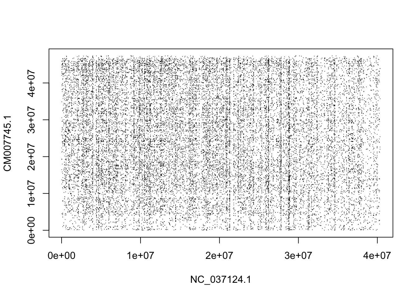

plot(dots,type="l")

OK, clearly what we have there is just a bunch of repetitive bits. I think we must not have the same chromosomes in the two species.

So, let’s put LG28 in coho against the whole chinook genome. Note the use of the bracketed “multiple” in there to let it know that there are multiple sequences in there that should get catenated together.

time lastz ~/Documents/UnsyncedData/Otsh_v1.0/Otsh_v1.0_genomic.fna[multiple]  coho-28.fna --notransition --step=20 --nogapped --ambiguous=iupac --format=maf > chin_vs_coho28.maf

FAILURE: in load_fasta_sequence for /Users/eriq/Documents/UnsyncedData/Otsh_v1.0/Otsh_v1.0_genomic.fna, sequence length 2,147,437,804+64,310 exceeds maximum (2,147,483,637)

No love there. But that chinook genome has a lot of short scaffolds in there too, I think.

Maybe we could just try LG1. Nope. How about we toss every coho LG against LG1 from chinook…

# let's get the first 10 linkage groups from coho:
for i in {1..10}; do curl ftp://ftp.ncbi.nlm.nih.gov/genomes/all/GCA/002/021/735/GCA_002021735.1_Okis_V1/GCA_002021735.1_Okis_V1_assembly_structure/Primary_Assembly/assembled_chromosomes/FASTA/chrLG${i}.fna.gz -o coho-${i}.fna.gz; gunzip coho-${i}.fna.gz; echo $i; done 

# now lets try aligning those to the chinook
for i in {1..10}; do time lastz chinook-1.fna coho-${i}.fna --notransition --step=20 --nogapped --ambiguous=iupac --format=rdotplot > chinook1_vs_coho${i}.rdp; echo "Done with $i"; done

Nothing looked good until I got to coho LG10:

dots <- readr::read_tsv("inputs/chinook1_vs_coho10.rdp.gz")

plot(dots,type="l")

There is clearly a big section that aligns there. But, we clearly are going to need to clean up all the repetive crap, etc on these alignments.

26.2.2 Try on the chinook chromosomes

So, it crapped out on the full Chinook fasta. Note that I could modify the code (or compile it with a -D): check this out in sequences.h:

//  Sequence lengths are normally assumed to be small enough to fit into a
//  31-bit integer.  This gives a maximum length of about 2.1 billion bp, which
//  is half the length of a (hypothetical) monoploid human genome.  The
//  programmer can override this at compile time by defining max_sequence_index
//  as 32 or 63.

But, for now, I think I will just go for the assembled chromosomes only:

# just get the well assembled chromosomes (about 1.7 Gb)
# in /tmp
samtools faidx ~/Documents/UnsyncedData/Otsh_v1.0/Otsh_v1.0_genomic.fna $(awk '/^NC/ {printf("%s ", $1)}'  ~/Documents/UnsyncedData/Otsh_v1.0/Otsh_v1.0_genomic.fna.fai) > chinook_nc_chroms.fna

# then try tossing coho 1 against that:
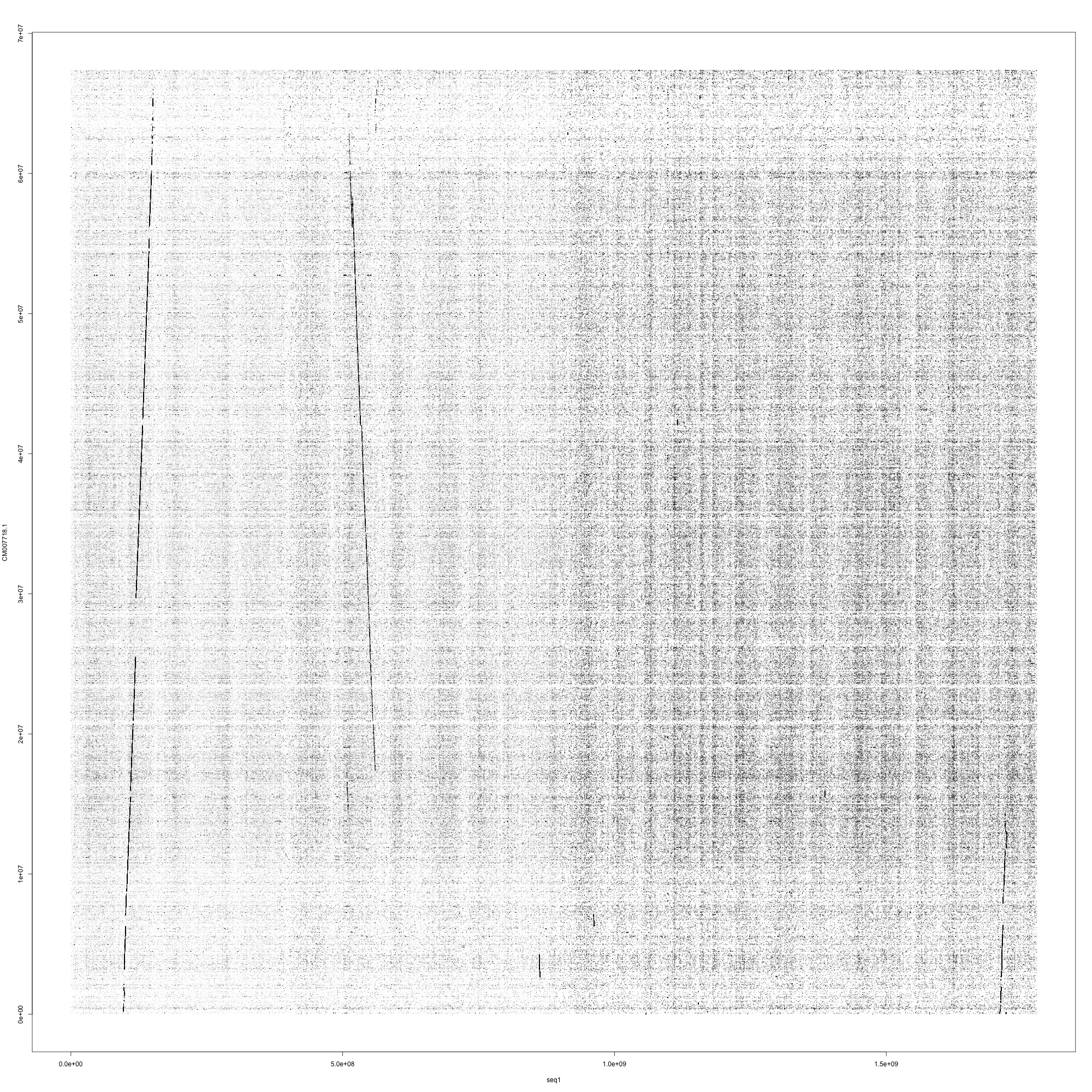
time lastz chinook_nc_chroms.fna[multiple]  coho-1.fna --notransition --step=20 --nogapped --ambiguous=iupac --format=rdotplot > chin_nc_vs_coho1.rdp

# that took about 7 minutes
real    6m33.411s
user    6m28.391s
sys 0m4.121s

Here is what the figure looks like. It is clear that the bulk of Chromosome 1 in coho aligns for long distances to two different chromosomes in Chinoook (likely paralogs?). This is complex!

Coho Chromo 1 on catenated chinook chromos

26.2.3 Explore the other parameters more

I am going to use the chinook chromosome 1 and coho 10 to explore things that will clean up the results a little bit.

# in /tmp
 i=10; time lastz chinook-1.fna coho-${i}.fna --notransition --step=20 --nogapped --ambiguous=iupac --format=rdotplot > chinook1_vs_coho${i}.rdp;
real    0m29.055s
user    0m28.497s
sys 0m0.413s

That is quick enough to explore a few things. Note that we are already doing gap-free extension, because “By default seeds are extended to HSPs using x-drop extension, with entropy adjustment.” However, by default, chaining is not done, and that is the key step in which a path is found through the high-scoring pairs (HSPs). That doesn’t take much (any) extra time and totally cleans things up.

i=10; time lastz chinook-1.fna coho-${i}.fna --notransition --step=20 --nogapped --ambiguous=iupac --format=rdotplot --chain  > chinook1_vs_coho${i}.rdp;

real    0m28.704s

So, that is greatly improved:

dots <- readr::read_tsv("inputs/chain-chinook1_vs_coho10.rdp.gz")

plot(dots,type="l")

So, it would be worth seeing if chaining also cleans up the multi-chrom alignment:

time lastz chinook_nc_chroms.fna[multiple]  coho-1.fna --notransition --step=20 --nogapped --ambiguous=iupac --format=rdotplot --chain > chin_nc_vs_coho1.rdp

real    6m42.835s
user    6m35.042s
sys 0m6.207s

dots <- readr::read_tsv("inputs/chin_nc_vs_coho1-chain.rdp.gz")

plot(dots,type="l")

OK, that shows that it will find crappy chains if given the chance. But if you zoom in on that stuff you see that some of the spots are pretty short, and some are super robust. So, we will want some further filtering to make this work. So, we need to check out the “back-end filtering.” that is possible. Back-end filtering does not happen by default.

Let’s say that we want 70 Kb alignment blocks. That is .001 of the total input sequence.

time lastz chinook_nc_chroms.fna[multiple]  coho-1.fna --notransition --step=20 --nogapped --ambiguous=iupac --format=rdotplot --chain --coverage=0.1 > chin_nc_vs_coho1-cov-0.1.rdp

That took 6.5 minutes again. But, it also produced no output whatsoever. We probably want to filter on identity first anyway. Because that takes so long, maybe we could do it with our single chromosome first.

i=10; time lastz chinook-1.fna coho-${i}.fna --notransition --step=20 --nogapped --ambiguous=iupac --format=rdotplot --chain  > chinook1_vs_coho${i}.rdp;

dots <- readr::read_tsv("/tmp/chinook1_vs_coho10-ident95.rdp")

plot(dots,type="l")

That keeps things very clean, but the alignment blocks are all pretty short (like 50 to 300 bp long). So perhaps we need to do gapped extension here to make these things better. This turns out to take a good deal longer.

i=10; time lastz chinook-1.fna coho-${i}.fna --notransition --step=20 --gapped --ambiguous=iupac --format=maf --chain --identity=95  > chinook1_vs_coho${i}-ident95-gapped.maf;

real    3m15.575s
user    3m14.048s
sys 0m0.936s

dots <- readr::read_tsv("/tmp/chinook1_vs_coho10-ident95-gapped.rdp")
plot(dots,type="l")

That is pretty clean and slick.

Now, this has got me to thinking that maybe I can do this on a chromosome by chromosome basis.

Check what 97% identity looks like:

i=10; time lastz chinook-1.fna coho-${i}.fna --notransition --step=20 --gapped --ambiguous=iupac --format=rdotplot --chain --identity=97  > chinook1_vs_coho${i}-ident97-gapped.rdp;

dots <- readr::read_tsv("/tmp/chinook1_vs_coho10-ident97-gapped.rdp")
plot(dots,type="l")

That looks to have a few more holes in it.

Final test. Let’s see what happens when we chain it on a chromosome that doesn’t have any homology:

# first with no backend filtering
i=1; time lastz chinook-1.fna coho-${i}.fna --notransition --step=20 --gapped --ambiguous=iupac --format=rdotplot --chain  > chinook1_vs_coho${i}-gapped.rdp;

real    0m35.130s
user    0m34.642s
sys 0m0.413s

# Hey! That is cool.  When there are no HSPs to chain, this doesn't take very long
i=1; time lastz chinook-1.fna coho-${i}.fna --notransition --step=20 --gapped --ambiguous=iupac --format=rdotplot --chain --identity=95 > chinook1_vs_coho${i}-gapped-ident95.rdp;

dots <- readr::read_tsv("/tmp/chinook1_vs_coho1-gapped.rdp")
plot(dots,type="l")

OK, it finds something nice and crappy there.

What about if we require 95% identity?

dots <- readr::read_tsv("/tmp/chinook1_vs_coho1-gapped-ident95.rdp")
plot(dots,type="l")

That leaves us with very little.

Let’s also try interpolation at the end to see how that does. Note that here we also produce the rdotplot at the same time as the maf.

i=10; time lastz chinook-1.fna coho-${i}.fna --notransition --step=20 --gapped --ambiguous=iupac --format=maf --rdotplot=chinook1_vs_coho${i}-ident95-gapped-inner1000.rdp --chain --identity=95 --inner=1000 > chinook1_vs_coho${i}-ident95-gapped-inner1000.maf;

real    4m25.625s
user    4m22.957s
sys 0m1.478s

That took an extra minute, but was not so bad.

dots <- readr::read_tsv("/tmp/chinook1_vs_coho10-ident95-gapped-inner1000.rdp")
plot(dots,type="l")

26.2.3.1 Repeat Masking the Coho genome

Turns out that NCBI site has the repeat masker output in GCF_002021735.1_Okis_V1_rm.out.gz. I save that to a shorter name. Now I will make a bed file of the repeat regions. Then I use bedtools maskfasta to softmask that fasta file.

# in: /Users/eriq/Documents/UnsyncedData/Okis_v1
gzcat Okis_V1_rm.out.gz | awk 'NR>3 {printf("%s\t%s\t%s\n", $5, $6, $7)}' > repeat-regions.bed 

bedtools maskfasta -fi Okis_V1.fna -bed repeat-regions.bed  -fo Okis_V1-soft-masked.fna  -soft

That works great. But it turns out that the coho genome is already softmasked.

But, it is good to now that I can use a repeat mask output file to toss repeat sites if I want to for ANGSD analyses, etc.

26.2.3.2 multiz maf2fasta

So, it looks like you can use single_cov2 from multiz to retain only a single alignment block covering each area. Then you can maf2fasta that and send it off in fasta format. Line2 holds the reference (target) sequence, but it has dashes added where the query has stuff not appearing in the target. So, what you have to do is run through that sequence and drop all the positions in the query that correspond to dashes in the target. That will get us what we want.

But maybe I can just use megablast like Christensen and company. They have some of their scripts, but it is not clear to me that it will be easy to get that back to a fasta for later analysis in ANGSD.

Not only that, but then there is the whole paralog issue. I am exploring that a little bit right now. It looks like when you crank the identity requirement up, the paralogs get pretty spotty so they can be easily recognized. For example setting the identity at 99.5 makes it clear which is the paralog:

time lastz chinook_nc_chroms.fna[multiple]  coho-1.fna --notransition --step=20 --nogapped --ambiguous=iupac --format=rdotplot --chain --identity=99.5 > chin_nc_vs_coho1-chain-ident-99.5.rdp
# takes about 6 minutes

And the figure is here.

Coho Chromo 1 on catenated chinook chromos. Ident=99.5

So, I think this is going to be a decent workflow:

1. run lastz on each coho linkage group against each chinook chromosome separately. Do this at identity=92 and identity=95 and identity=99.9. For each run, produce a .maf file and at the same time a .rdotplot output.
2. Combine all the .rdotplot files together into something that can be faceted over chromosomes and make a massive facet grid showing the results for all chromosomes. Do this at different identity levels so that the paralogs can be distinguished.
3. Visually look up each columns of those plots and determine which coho chromosomes carry homologous material for each chinook chromosome. For each such chromosome pair, run single_cov2 on them (maybe on the ident=92 version).
4. Then merge those MAFs. Probably can just cat them together, but there might be some sorting that needs to be done on them.
5. Run maf2fasta on those merged mafs to get a fasta for each chinook chromosome.
6. Write a C-program that uses uthash to efficiently read the fasta for each chinook chromosome and then write out a version in which the positions that are dashes in the chinook reference are removed from both the chinook reference and the aligned coho sequence. _Actually, one can just pump each sequence out to a separate file in which each site occupies one line. Then paste those and do the comparison…

2018-10-18 11:15 /tmp/--% time (awk 'NR==2' splud | fold -w1 > spp1.text)

real    0m23.244s
user    0m22.537s
sys 0m0.685s

# then you can use awk easily like this:
paste spp1.text spp2.text | awk 'BEGIN {SUBSEP = " "} {n[$1,$2]++} END {for(i in n) print i, n[i]}' 

7. The coho sequence thus obtained will have dashes anywhere there isn’t coho aligned to the chinook. So, first, for each chromosome I can count the number of dashes, which will tell me the fraction of sites on the chinook genome that were aligned (sort of—there is an issue with N’s in the coho genome.) Then those dashes can be converted to N’s.
8. It would be good to count the number of sites that are not N’s in chinook that are also not Ns in coho, to know how much of it we have aligned.

Note, the last thing that really remains here is making sure that I can run two or more different query sequences against one chinook genome and then process that out correctly into a fasta.

Note that Figure 1 in christensen actually gives me a lot to go on in terms of which chromosomes in coho to map against which ones in chinook.