Chapter 10 A Tidy Approach to Spatial Data: Simple Features

Note that if you, the student, wish to run all the code yourself, you should download the inputs directory as a zipped file by going here with a web browser and then clicking the big “Download” button on the right. Once you have downloaded that, unzip it and put the whole inputs directory in the current working directory where you are working with R.

10.1 Prelims

If you don’t already have it:

install.packages("sf")

Also, as of June 5, 2017, this requires the development version of ggplot2:

devtools::install_github("tidyverse/ggplot2")

Be warned that this seems to break some of the earlier ggmap.

library(tidyverse)
library(sf)

## Linking to GEOS 3.4.2, GDAL 2.1.2, proj.4 4.9.1

library(raster)

10.2 Reading spatial data into sf objects

Let’s just quickly put the code in to reproduce most of the stuff from the previous lecture, but using sf.

Note that there are two functions to read shapefiles: st_read() and read_sf(). The latter seems preferable to me as it does not read stringsAsFactors ever.

streams <- read_sf("inputs/santa-cruz-county/Streams/Streams.shp")
watersheds <- read_sf("inputs/santa-cruz-county/Watersheds/Watersheds.shp")
lights <- read_sf("inputs/santa-cruz-county/Street_Lights/Street_Lights.shp")

Have a look at one of them. Note that the whole thing is a data frame, so you can directly as_tibble() it:

as_tibble(streams)

## # A tibble: 1,514 x 9
##    OBJECTID       STREAM_NM   STREAMTYPE  GNIS_ID    ID ENABLED Named
##       <dbl>           <chr>        <chr>    <chr> <chr>   <chr> <chr>
##  1        1     Adams Creek INTERMITTENT     <NA>     0    <NA>   Yes
##  2        2      Alba Creek    PERENNIAL 00218063     1    <NA>   Yes
##  3        3     Amaya Creek    PERENNIAL 00218217     2    <NA>   Yes
##  4        4 Ano Nuevo Creek    PERENNIAL 00254567     3    <NA>   Yes
##  5        5     Aptos Creek    PERENNIAL 00254571     4    <NA>   Yes
##  6        6 Archibald Creek INTERMITTENT 00218350     5    <NA>   Yes
##  7        7   Baldwin Creek    PERENNIAL 00218614     6    <NA>   Yes
##  8        8     Bates Creek    PERENNIAL 00218726     7    <NA>   Yes
##  9        9      Bean Creek    PERENNIAL 00218782     8    <NA>   Yes
## 10       10   Bennett Creek    PERENNIAL 00219040     9    <NA>   Yes
## # ... with 1,504 more rows, and 2 more variables: SHAPESTLen <dbl>,
## #   geometry <simple_feature>

10.3 Plotting sf objects

In ggplot this is made easy with the geom_sf() which knows what type of simple feature you have, and plots it appropriately.

You also add coord_sf() which will deal with projections, on the fly, and also takes care of aspect ratios and draws a graticule.

ggplot() +
  geom_sf(mapping = aes(colour = STREAMTYPE), data = streams) +
  coord_sf()

Check it out, there is a graticule. Note that the long-lat lines are not perfectly square. That is because this object is not in long-lat:

st_crs(streams)

## $epsg
## [1] NA
## 
## $proj4string
## [1] "+proj=lcc +lat_1=37.06666666666667 +lat_2=38.43333333333333 +lat_0=36.5 +lon_0=-120.5 +x_0=2000000 +y_0=500000.0000000002 +datum=NAD83 +units=us-ft +no_defs"
## 
## attr(,"class")
## [1] "crs"

Aha! See, it is in lcc = lambert conic conformal.

What happens if we try to put an open street maps on this? It fails…

How about if we try to use spraster_rgb to put a raster background in there? That is a little complicated. So, instead let’s have a look at interactive mapping later.

But before that I want to briefly touch on geometrical intersections.

10.4 Geometric operations

Just briefly, remember, we wondered last week how to find all the streams that are in the Scott Creek watershed. This can be done with the raster package, nicely. But with the sf package we can also use st_intersection() to spatially intersect streams with watersheds. When we do this, the cool thing is that all the columns of data associated with each get joined just as you would hope they do!!

streamsheds <- st_intersection(streams, watersheds)

## Warning: attribute variables are assumed to be spatially constant
## throughout all geometries

Those columns get joined on the basis of the stream being in the watershed. Cool!

Check it out:

as_tibble(streamsheds)

## # A tibble: 1,522 x 15
##    OBJECTID         STREAM_NM   STREAMTYPE  GNIS_ID    ID ENABLED Named
##  *    <dbl>             <chr>        <chr>    <chr> <chr>   <chr> <chr>
##  1        4   Ano Nuevo Creek    PERENNIAL 00254567     3    <NA>   Yes
##  2       25     Cascade Creek    PERENNIAL 00220660    24    <NA>   Yes
##  3       38      Elliot Creek    PERENNIAL 00223153    37    <NA>   Yes
##  4       41      Finney Creek    PERENNIAL 00223512    40    <NA>   Yes
##  5       47       Gazos Creek    PERENNIAL     <NA>    46    <NA>   Yes
##  6       51  Green Oaks Creek    PERENNIAL 00224554    50    <NA>   Yes
##  7       91  Old Womans Creek    PERENNIAL 00229991    90    <NA>   Yes
##  8      129 White House Creek    PERENNIAL     <NA>   128    <NA>   Yes
##  9      131      Willow Gulch INTERMITTENT     <NA>   130    <NA>   Yes
## 10      162       Stream 1141        SWALE     <NA>   161    <NA>    No
## # ... with 1,512 more rows, and 8 more variables: SHAPESTLen <dbl>,
## #   OBJECTID.1 <dbl>, NAME <chr>, COUNT_ <dbl>, MapKey <chr>,
## #   SHAPESTAre <dbl>, SHAPESTLen.1 <dbl>, geometry <simple_feature>

Plot it with different colors for different watersheds to see what I mean:

ggplot(streamsheds) +
  geom_sf(aes(colour = NAME)) +
  coord_sf()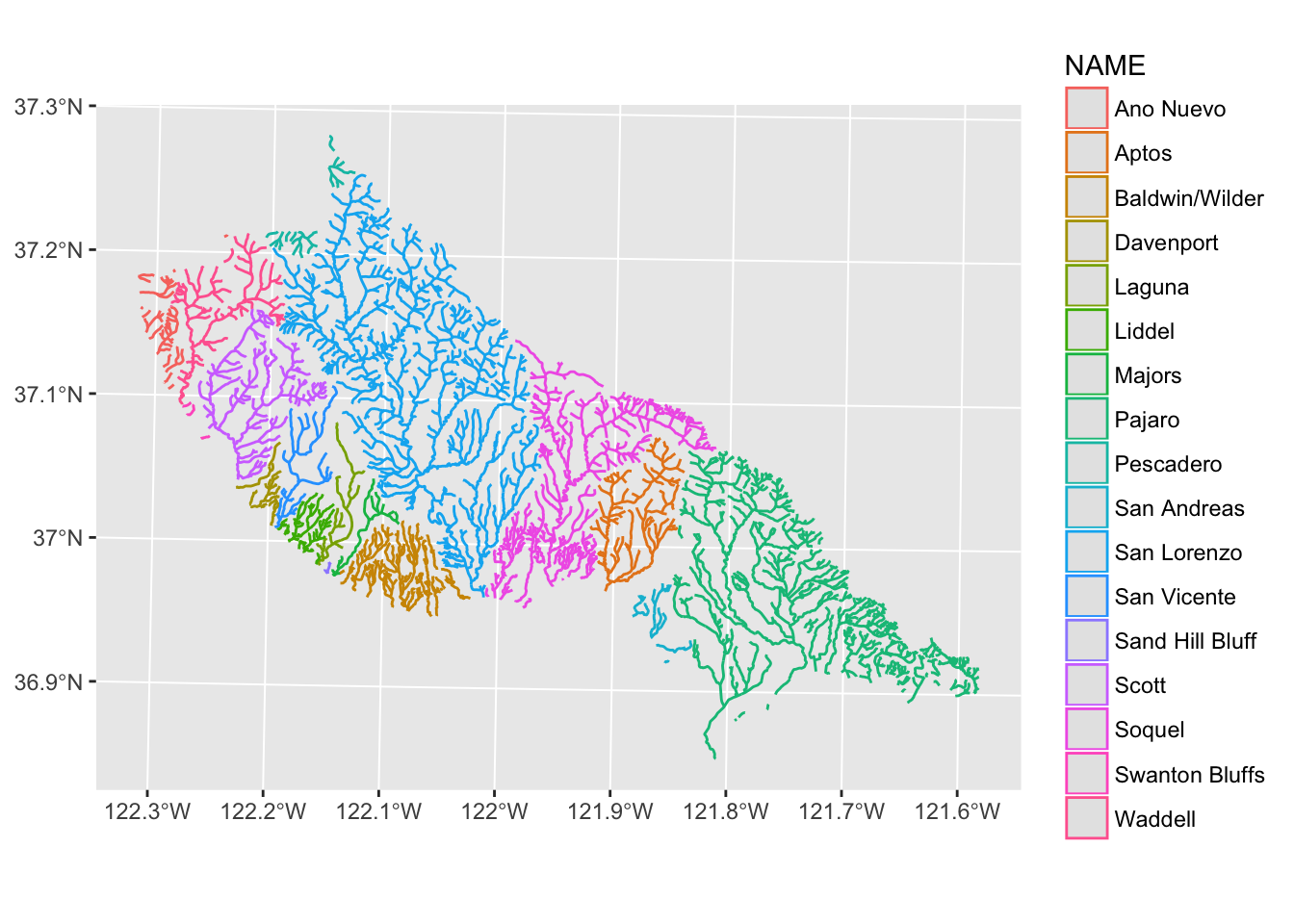

OK, now let’s make some interactive maps.

10.5 Interactive plotting with leaflet via the mapview package

This is truly mind-blowing. The authors of the mapview package tell us:

“mapview is an R package created to help researchers during their spatial data analysis workflow. It provides functions to very quickly and conveniently create interactive visualisations of spatial data. It was created to fill the gap of quick (not presentation grade) interactive plotting to examine and visually investigate both aspects of spatial data, the geometries and their attributes.”

As such, it appears that customization of certain things might not be easily-accessible, but it is so easy and still so customizable that it is really, really amazing.

Get it from CRAN:

install.packages("mapview")

and then be sure to load it:

library(mapview)

## Loading required package: leaflet

The main function is mapView which does multiple dispatch on a huge variety of different object types (rasters, points, polygons, etc), including sf classes. It creates an interactive web-map powered by leaflet, an open-source JavaScript library for mobile-friendly interactive maps.

Let’s look at it in action:

mapView(streams)

Some control elements you should note:

• Upper left zoom in and out “+/-”
• Below that is the layer selector. Choose your background and which layers to show
• Lower right is the “fit this layer in the view” button. Move the map, then try it.

Also, mouse over some streams and click on them. Far out! All that information at your fingertips!

10.5.1 Mapping attributes

What if we want to map STREAMTYPE to color? We use the zcol argument for this. And we can use map.types to give a string that names what type of background map we want. From the help file you see that the map.types can be previewed at: http://leaflet-extras.github.io/leaflet-providers/preview/.

mapView(streams, map.type = "Esri.WorldShadedRelief", zcol = "STREAMTYPE")

10.5.2 Adding layers

This is done by using the “+” symbol, much as in ggplot. Here we will put the watersheds down first with rainbow fill colors for the different watersheds (and white perimeters), then we will put the streams on top of that, and finally we will through down some streetlights. We will also put legends down for the watersheds and the streams.

sc_map <- mapView(watersheds, 
        map.type = "Esri.WorldShadedRelief", 
        zcol = "NAME", 
        col.regions = rainbow(7), 
        color = "white",
        legend = TRUE) +
  mapView(streams, zcol = "STREAMTYPE", legend = TRUE) +
  mapView(lights)

sc_map

10.5.3 Saving maps

Truth by told, the bookdown format is a little narrow to allow a nice large map. But you can save it as a web page with mapshot and then size it up in your browser. For example:

mapshot(sc_map, url = "/tmp/my_map.html")

Or, if you are just working in RStudio, the things render just fine in the preview window, and then you can zoom it as a separate page.

You can also save static pdf, png, or jpg files:

mapshot(sc_map, file = "/tmp/sc_map.pdf")

10.6 Adding map tiles from other sources

This blog post just came up today, talking about how to hack more types of map tiles from avaible WMS servers. (From Wikipedia: A Web Map Service (WMS) is a standard protocol for serving (over the Internet) georeferenced map images which a map server generates using data from a GIS database. The Open Geospatial Consortium developed the specification and first published it in 1999.)

It turns out that there is a WMS for the tasty NOAA shaded color mosaic that we used for Carmel Bay last week.

So, lets see if we can use jimbob’s post to plot (a sample of) Diana’s rockfish data on top of those tiles.

First we are going to sample 2000 fish into a simple features data frame, and then pretend we know the species of them

# get our rockfish location data and add species pseudo data on them
set.seed(5)
seb <- readRDS("inputs/sebastes_locations.rds") %>%
  filter(!is.na(LONGITUDE_M) & !is.na(LATITUDE_M)) %>%
  filter(LONGITUDE_M < -121.75117) %>% # some of the the longitudes are missing their minus sign
                                       # and a few others are wrong---in the Salinas Valley!
  sample_n(2000) %>%
  mutate(species = sample(c("kelp", "gopher", "black-and-yellow", "copper"), 2000, replace = TRUE))

# make an sf object of that
seb_sf <- st_as_sf(seb, 
                   coords = c("LONGITUDE_M", "LATITUDE_M"),
                   crs = (4326))  # this is a longlat coord ref system

Then we can make a standard leaflet map of that, coloring by (fake) species.

seb_map <- mapView(seb_sf, zcol = "species", legend = TRUE)
seb_map

That is pretty darn cool just like that.

But now, I have dredged up the URL for the WMS for the NOAA global mosaic hillshade. And we can stick that into the following code:

seb_map@map <- seb_map@map %>% 
  addWMSTiles(group = "NOAA_mosaic",
              baseUrl = "https://gis.ngdc.noaa.gov/arcgis/services/DEM_global_mosaic_hillshade/ImageServer/WMSServer?",
              layers = "0",
              attribution = '<a href="http://www.noaa.gov">NOAA</a>') %>%   # a link to NOAA for the map
  mapview:::mapViewLayersControl(names = c("NOAA_mosaic"))

# then print it
seb_map

10.7 More info

This has been a whirlwind. Interested parties should definitely read about:

• Simple Features Vignette
• Online vignettes for mapview

For more on leaflet for R, see: - Leaflet for R