Session 7 Genetic and Environmental Associations

7.1 Background

Now that we know how to get environmental layers and plot them in space, for many of the species we are working on, we are not entirely sure which environmental variables are important drivers of populaiton genetic structure or underlying phenotypic traits of interest.

Let’s back up. Now, we have access to multiple layers of environmental layers that span a species range:

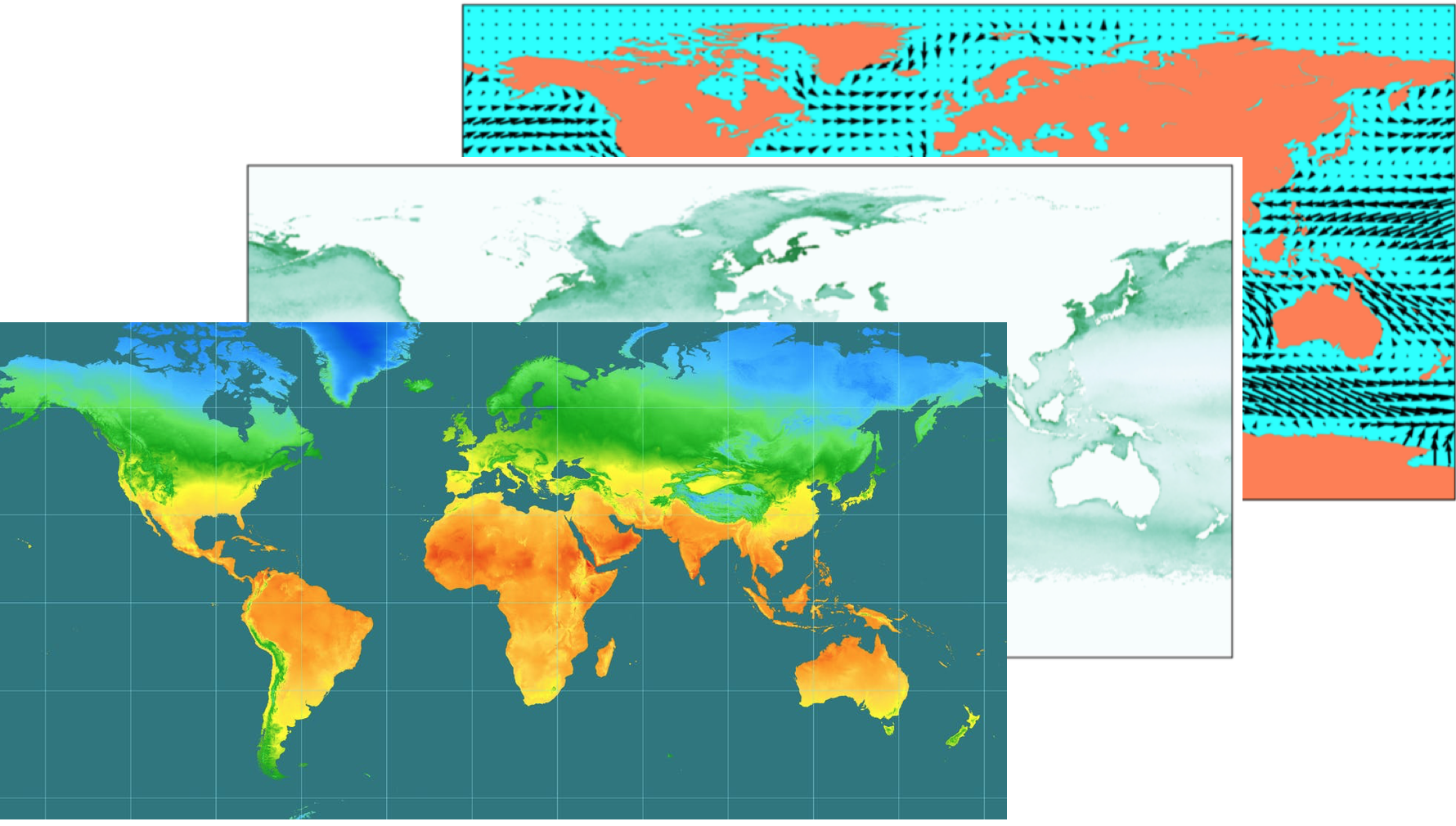
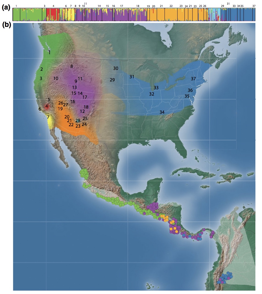
And many of us now have genomic data. Here, we used genome-wide reduced representation sequencing to create a spatially explicit map of population structure, called the genoscape, of the Willow Flycatcher.

What we ultimately want to investigate is how environmental variables are correlated with genetic variation.

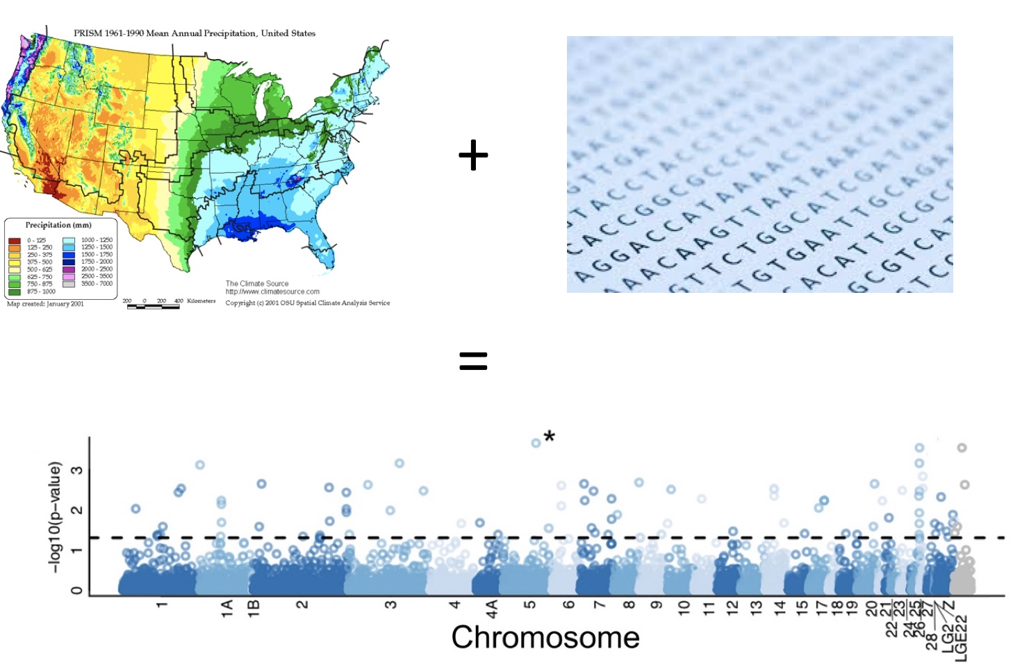
Standing genetic variation associated with current climate gradients theoretically indicates adaptive capacity. However, modeling future adaptation from individual loci is difficult because we don’t understand all GxE interactions.

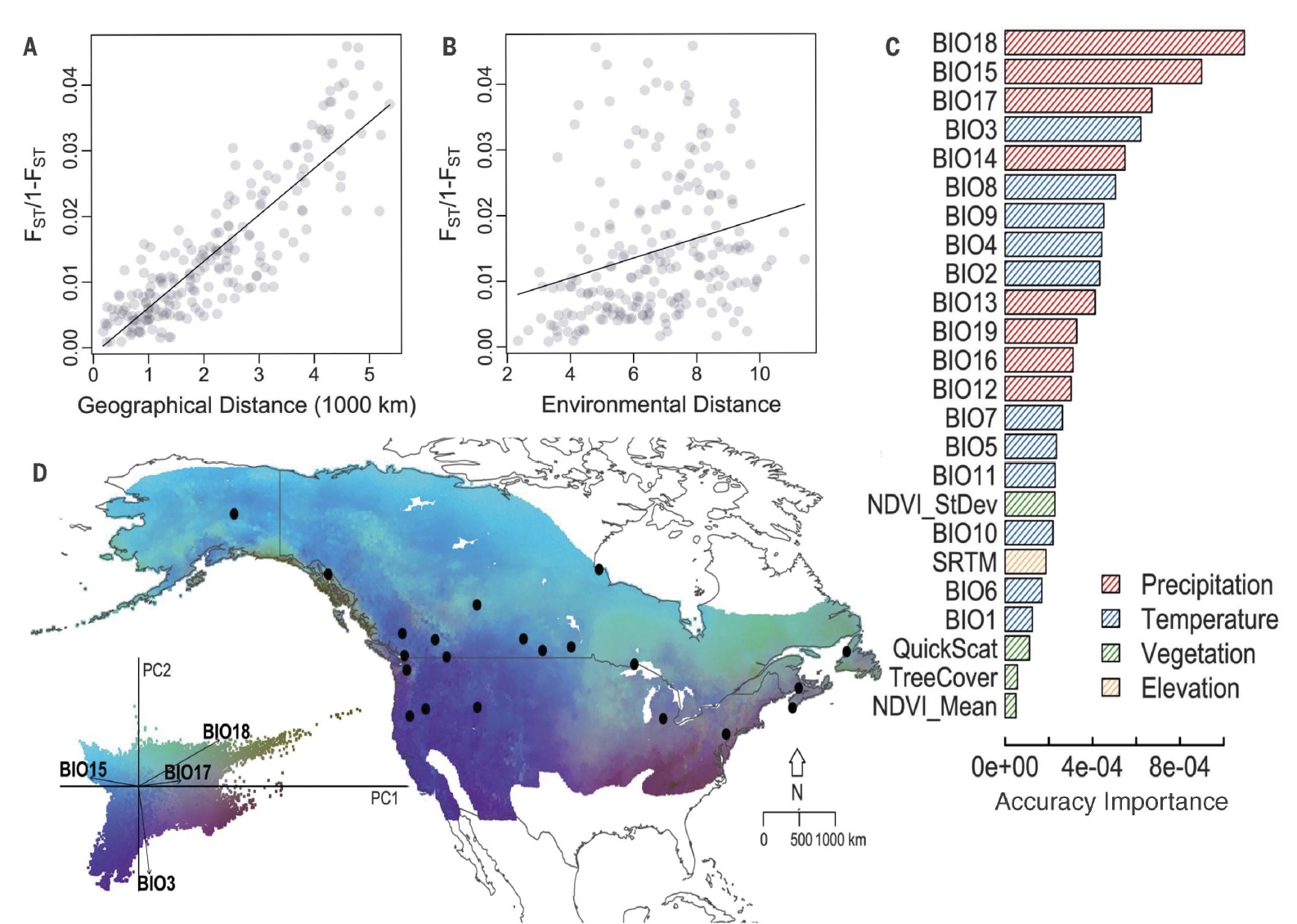
A recent example illustrated that not only is geography (“isolation by distance”) strongly correlated genetic structure, but environment plays a role in differentiation too. Specifically, precipitation is a strong predictor of Yellow Warbler genetic structure.

7.2 Motivation

The R package gradientForest traditionally quantifies multi-species compositional turnover along environmental gradients. In the era of next-generation sequencing, where genome-wide data is common, we can extend this community ecology framework to determine which variants are associated with specific environmental variables. So rather than thinking of the large-scale species turnover in space, we can map fine-scale allele frequency changes along environemntal gradients.

Gradient forest is a machine learning approach for classification and regression based on decision trees. We’ve all seen and used decision trees, for mundane tasks like waking up to an alarm each morning to more intricate decisions like optimal pairing of individuals in a captive breeding program to increase/maintain genetic diversity of a population. Regardless of which decision tree you are implementing, the assumption remains, the higher the split, the more important the predictor.

Because decision trees are prone to overiftting, gradient forest uses random forests to test associations. Random forests use a random subset of predictors for each decision tree.

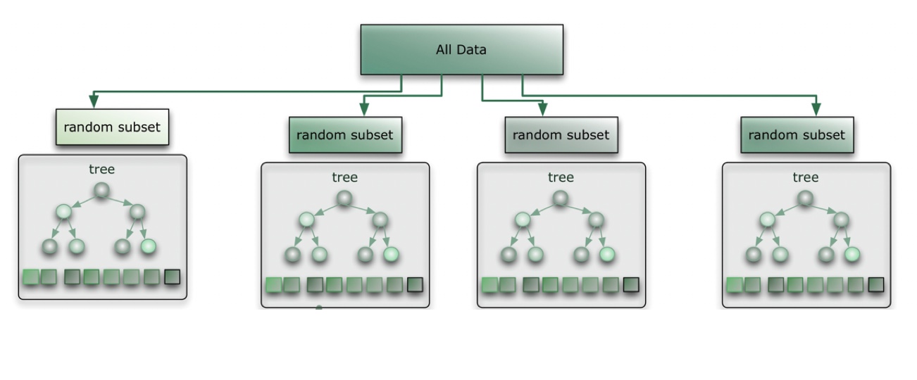
1. Choose a subset of data and predictors.
2. Find predictor (and value) that optimizes split.
3. Create many trees and aggregate.

Random forests and genomic data

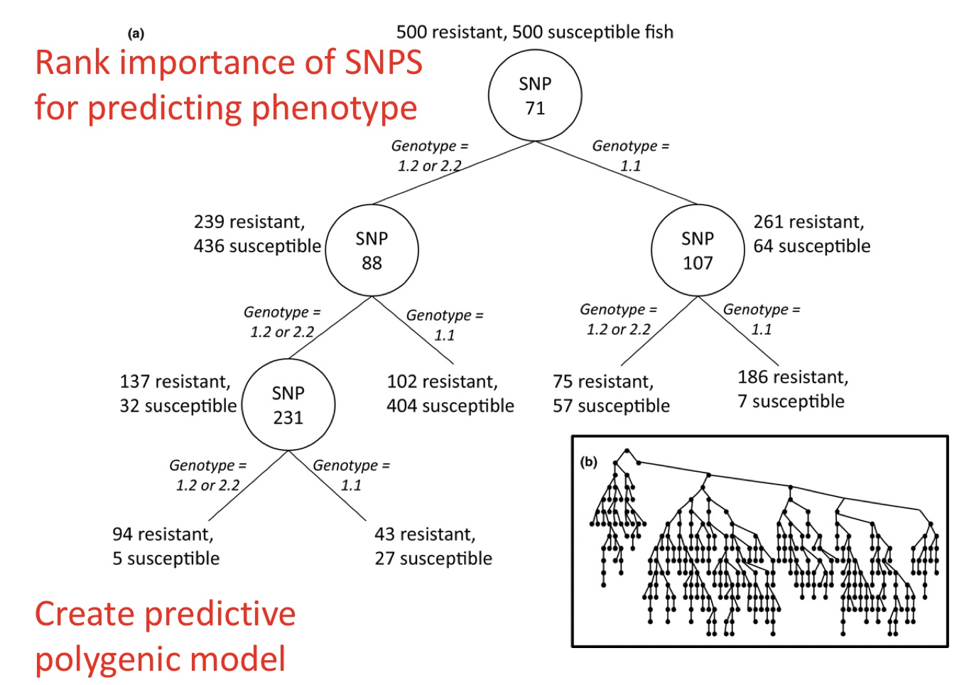
Brieuc et al. 2018 used this approach to rank the importance of SNPs for predicting a specific binary phenotype, e.g. disease resistance in fish. This is an example of one random tree, which can ultimately create a predictive polygenic model.

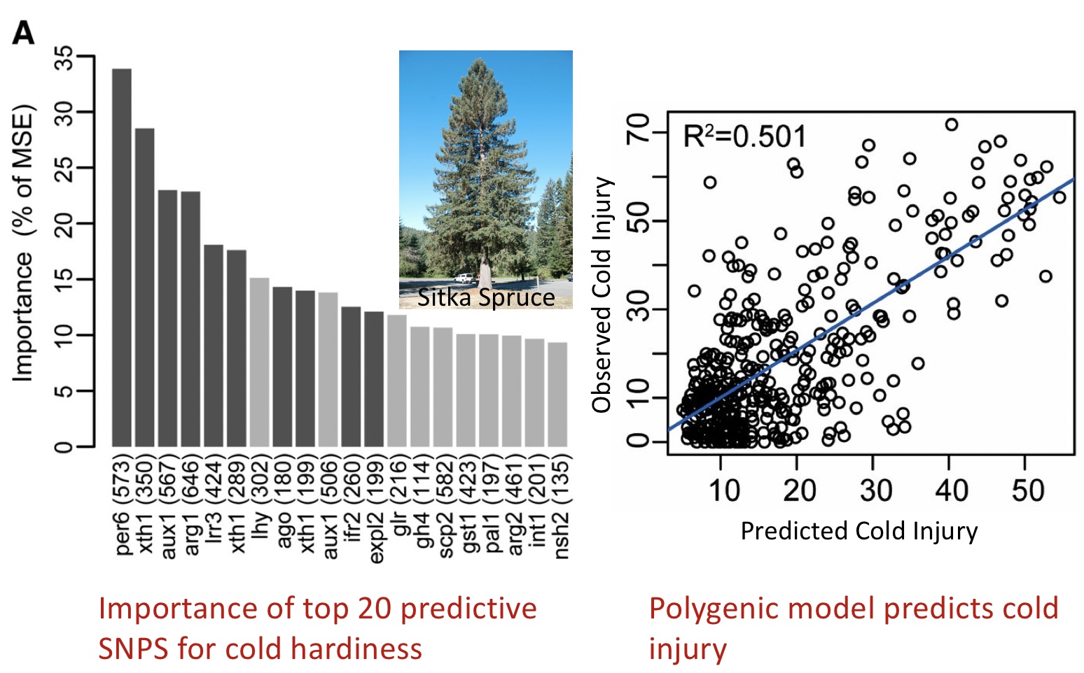
Another interesting study used random forests to find the predictive variants for cold hardiness, which was subsequently used to predict cold injury in the Sitka Spruce (Holliday et al. 2012).

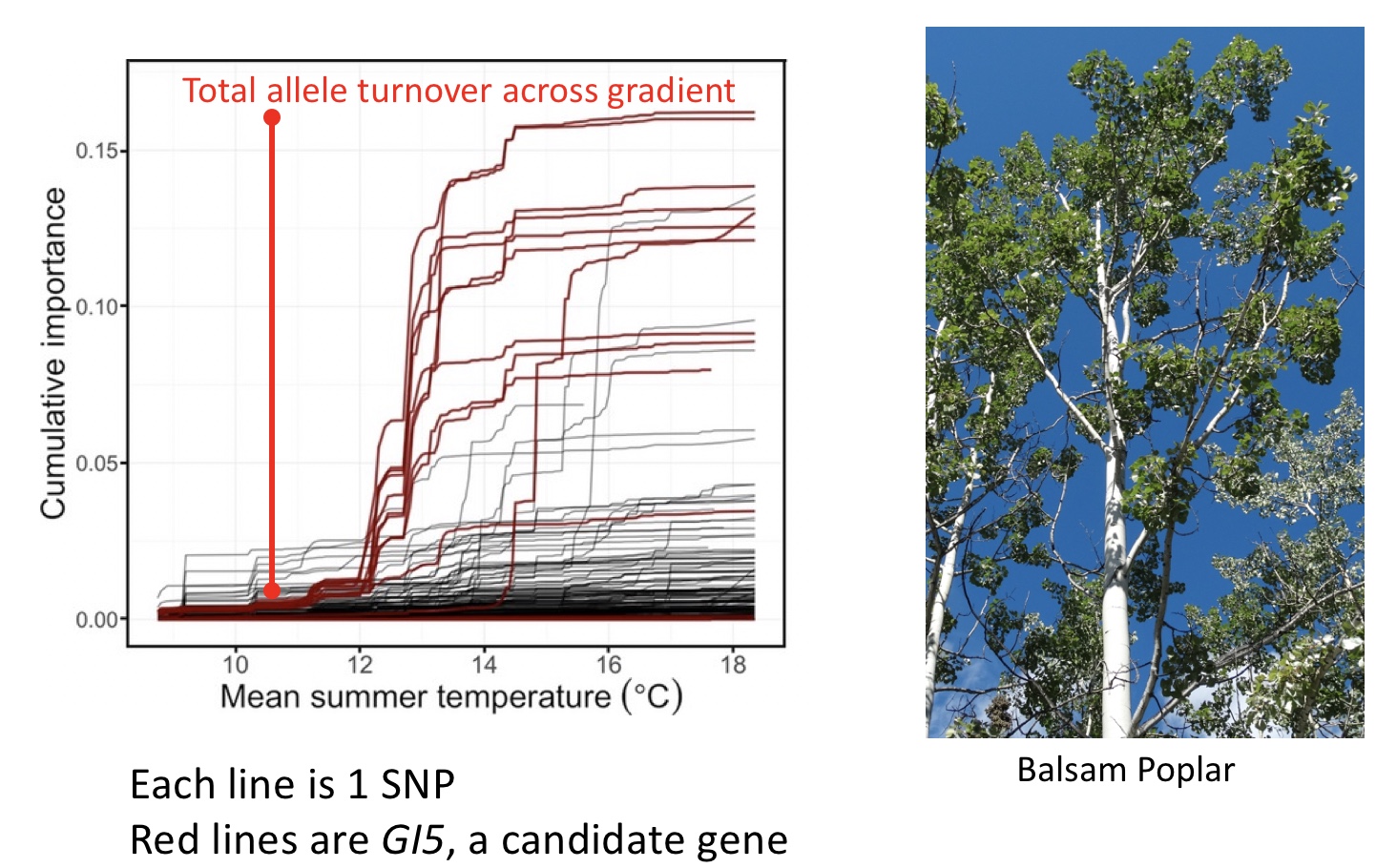
What if we have multiple SNPs AND multiple phenotypes or environments? Gradient forest extends random forest to incorporate multiple response variables.

Gradient uses turnover functions to look at total allele turnover across environmental gradients. For instance, GI5, a candidate gene in Balsam Poplar, clearly shows great allele frequency transitions across the mean summer temperature (Fitzpatrick and Keller 2015)

If we look at different subsets of genetic variation in Balsam Poplar space

1. reference SNPs,
   
2. GI5, a candidate gene for genetic control of bud set and bud flush (Olson et al. 2013)

you can see that different environmental variables predict genetic variation of the reference and candidate genes. Note different colors = locally adapted genotypes.

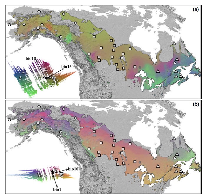
Below is code for quantifying and visualizing intraspecific gene-environment variation across space. As part of The Bird Genoscape Project, we compare present-day gene-environment associations to predicted future changes to identify regions of genomic vulnerability.

For now, this tutorial focuses on analyzing and plotting the allelic variation as estimated from gradient forest for a single species, the Willow Flycatcher, but is easily adpated to include other species and methods for esimating variation.

7.3 Housekeeping

We will need the following R packages. gradientForest requires the dependancy extendedForest, an R package classification and regression based on forest trees using random inputs. With the newest version of R, extended forest is installed automatically as a dependency.

Install and load the following packages in Rstudio. You can use the Packages function to the right to install most packages except for gradient forest, which we will install from R-Forge.

1. As discussed in Setting Up Your Computer, if you have a Mac, you will need the XCode command line tools.
2. If you have a PC, you’ll need Rtools
3. You will also need gfortran on your computer. See the instructions in Setting Up Your Computer if you don’t have that set up already.

Also, you need to have the package ‘gradientForest’ installed as described in the Preface section The ‘gradientForest’ package.

#install.packages("gradientForest", repos="http://R-Forge.R-project.org")
library(gradientForest)
library(data.table)

## 
## Attaching package: 'data.table'

## The following objects are masked from 'package:terra':
## 
##     copy, shift

## The following objects are masked from 'package:dplyr':
## 
##     between, first, last

## The following object is masked from 'package:purrr':
## 
##     transpose

library(raster)

## Loading required package: sp

## 
## Attaching package: 'raster'

## The following object is masked from 'package:dplyr':
## 
##     select

library(gstat)
library(rgdal)

## Please note that rgdal will be retired by the end of 2023,
## plan transition to sf/stars/terra functions using GDAL and PROJ
## at your earliest convenience.
## 
## rgdal: version: 1.5-28, (SVN revision 1158)
## Geospatial Data Abstraction Library extensions to R successfully loaded
## Loaded GDAL runtime: GDAL 3.2.1, released 2020/12/29
## Path to GDAL shared files: /Library/Frameworks/R.framework/Versions/4.1/Resources/library/rgdal/gdal
## GDAL binary built with GEOS: TRUE 
## Loaded PROJ runtime: Rel. 7.2.1, January 1st, 2021, [PJ_VERSION: 721]
## Path to PROJ shared files: /Library/Frameworks/R.framework/Versions/4.1/Resources/library/rgdal/proj
## PROJ CDN enabled: FALSE
## Linking to sp version:1.4-6
## To mute warnings of possible GDAL/OSR exportToProj4() degradation,
## use options("rgdal_show_exportToProj4_warnings"="none") before loading sp or rgdal.
## Overwritten PROJ_LIB was /Library/Frameworks/R.framework/Versions/4.1/Resources/library/rgdal/proj

## 
## Attaching package: 'rgdal'

## The following object is masked from 'package:terra':
## 
##     project

library(sf)
library(RColorBrewer)
library(rasterVis)

## Loading required package: lattice

library(tidyverse)

And we will need to load a realistic, polygon shapefile (an outline of the Willow Flycatcher’s breeding range in North America for this exercise) and set its projection. Note, you will need to adjust the path to the shapefile below. This is the path to my shape file on my computer.

That will produce this map:

wifl_shape <-st_read("data/6.0/WIFLrev.shp")

## Reading layer `WIFLrev' from data source 
##   `/Users/eriq/Documents/git-repos/merida-workshop-2022/data/6.0/WIFLrev.shp' 
##   using driver `ESRI Shapefile'
## Simple feature collection with 5 features and 14 fields
## Geometry type: MULTIPOLYGON
## Dimension:     XY
## Bounding box:  xmin: -128.4 ymin: 29.04 xmax: -67.01 ymax: 53.46
## Geodetic CRS:  WGS 84

ggplot(wifl_shape) +
  geom_sf(fill=NA) +
  theme_bw()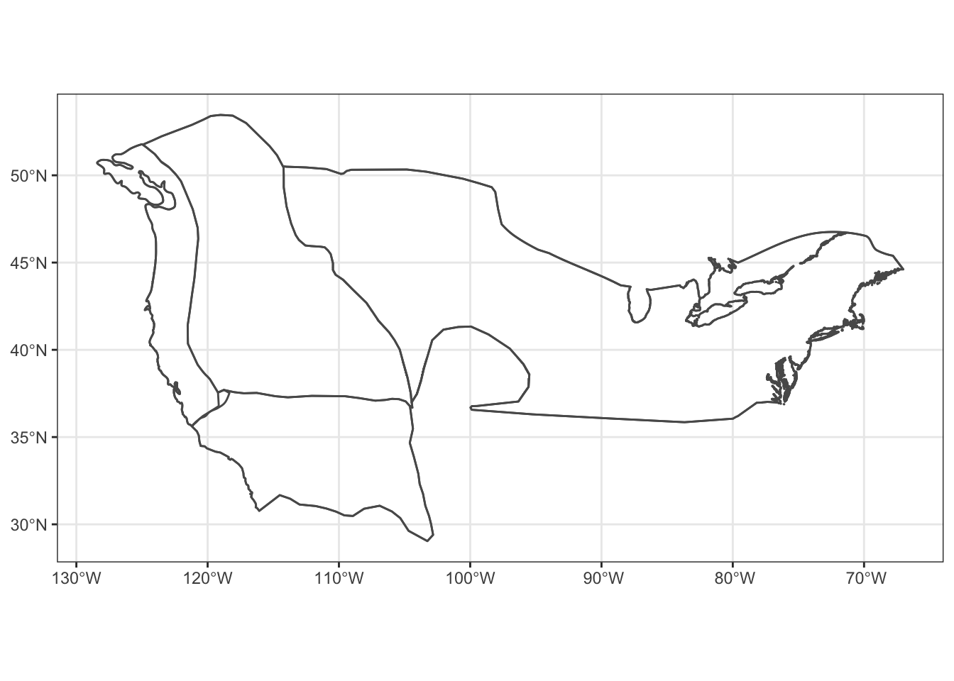

FIGURE 7.1: A basic outline of Willow Flycatcher breeding range we will use for this exercise

7.4 Running Gradient Forest

We will use gradient forest to test whether a subset of genomic variation can be explained by environmental variables and to visualize climate-associated genetic variation across the breeding range of the Willow Flycatcher. To run gradient forest we need two main files. First we need the environmental data/climate variables associated with each population. Populations are defined by their latitude and longitude.

For each sampling location, we obtained environmental data from publically available databases. Specifically, we chose variables with known impacts on bird physiology and ecology and that were publically available at high resolution. These variables included 19 climate variables downloaded from WorldClim (Hijmans et al. 2005) as well as vegetation indices (Carroll et al. 2004) (NDVI and NDVIstd), Tree Cover (Sexton et al. 2013) and elevation data from the Global Land Cover Facility (http://www.landcover.org). We also downloaded and used a measure of surface moisture characteristics from the NASA Scatterometer Climate Record Pathfinder project (QuickSCAT, downloaded from scp.byu.edu).

Read in the environmental variables, and take a look at the dimensions and the actual data.

Ewifl<-read_csv('data/6.0/wiflforest.env.csv')

## Rows: 21 Columns: 23

## ── Column specification ───────────────────────────────
## Delimiter: ","
## dbl (23): BIO1, BIO2, BIO3, BIO4, BIO5, BIO6, BIO7,...

## 
## ℹ Use `spec()` to retrieve the full column specification for this data.
## ℹ Specify the column types or set `show_col_types = FALSE` to quiet this message.

dim(Ewifl)

## [1] 21 23

How many sites do we have environmental data for? How many environmental variables?

Gradient forest does not directly account for spatial population structure. But there are some possible ways to deal with this:

• Include Lat/Long as predictors.

• Moran’s Eigenvector Map (MEM) variables – spatial eigenvectors (Fitzpatrick et al. 2015)

• ”regress out” population cluster membership (Holliday et al. 2012 did this for phenotypes).

• Use genomic PCAs as predictors (Exposito-Alonso et al. 2018)

Your choice depends on the biology of your organism and your question. You’ll notice in this tutorial, by examining the environmental data we are using in the code chunk below, we do not account for population structure.

head(Ewifl)

## # A tibble: 6 × 23
##    BIO1  BIO2  BIO3  BIO4  BIO5  BIO6  BIO7  BIO8  BIO9
##   <dbl> <dbl> <dbl> <dbl> <dbl> <dbl> <dbl> <dbl> <dbl>
## 1   193   165    43  7888   392    15   377    95   227
## 2   205   165    44  7792   395    23   372   300   242
## 3    52   180    50  6365   237  -116   353   131    78
## 4    86   166    47  6468   290   -63   353    13   171
## 5   168   107    54  3298   265    65   200   132   206
## 6   166   158    44  7032   360     4   356    94   258
## # … with 14 more variables: BIO10 <dbl>, BIO11 <dbl>,
## #   BIO12 <dbl>, BIO13 <dbl>, BIO14 <dbl>,
## #   BIO15 <dbl>, BIO16 <dbl>, BIO17 <dbl>,
## #   BIO18 <dbl>, BIO19 <dbl>, NDVI_Mean <dbl>,
## #   NDVI_StDev <dbl>, SRTM <dbl>, TreeCover <dbl>

Second, we have genomic data formatted as allele frequencies for each population in the same order. The published Willow Flycatcher data includes 37855 variants, and is too large to run a gradient forest analyses within the time frame of a tutorial, so we are supplying a subsetted dataset limited to 10,000 SNPs.

Gwifl<-read_csv('data/6.0/wiflforest.allfreq.sample.csv')

## Rows: 21 Columns: 10000

## ── Column specification ───────────────────────────────
## Delimiter: ","
## dbl (10000): V21252, V9139, V22510, V5860, V3386, V...

## 
## ℹ Use `spec()` to retrieve the full column specification for this data.
## ℹ Specify the column types or set `show_col_types = FALSE` to quiet this message.

dim(Gwifl)

## [1]    21 10000

head(Gwifl)

## # A tibble: 6 × 10,000
##   V21252  V9139 V22510 V5860 V3386 V14932 V14581  V9277
##    <dbl>  <dbl>  <dbl> <dbl> <dbl>  <dbl>  <dbl>  <dbl>
## 1  0.15  0.333  0.25   0.45  0.3    0.3    0.4   0.125 
## 2  0.107 0.25   0.25   0.571 0.308  0.607  0.357 0.143 
## 3  0.115 0.231  0.167  0.654 0.308  0.208  0.192 0.136 
## 4  0     0.1    0.0833 0.667 0.417  0.167  0     0.1   
## 5  0.25  0.667  0.125  0.625 0      0.75   0.25  0     
## 6  0.192 0.0833 0.0385 0.115 0.192  0.269  0.154 0.0909
## # … with 9,992 more variables: V25872 <dbl>,
## #   V23716 <dbl>, V25026 <dbl>, V11453 <dbl>,
## #   V2266 <dbl>, V371 <dbl>, V21324 <dbl>,
## #   V28422 <dbl>, V8773 <dbl>, V5906 <dbl>,
## #   V15909 <dbl>, V20940 <dbl>, V15435 <dbl>,
## #   V9026 <dbl>, V12438 <dbl>, V2181 <dbl>,
## #   V23539 <dbl>, V19510 <dbl>, V15571 <dbl>, …

These are allele frequencies for each site. What is the range of allele frequencies for allele V3386? You might need to write extra code to answer this question.

Next we have some housekeeping to define the predictor variables in the regression, which are the environmental variables, and the response variables, which in this case are the frequencies of each variant, analyzed in gradient forest.

Another variable in the gradientForest model is maxLevel, which we define using an equation recommended by gradient forest.

# set depth of conditional permutation
lev <- floor(log2(nSites*0.368/2))
lev

## [1] 1

First, and notably, predictor variables are often correlated. The standard approach in random forests assesses marginal importance of predictor by randomly permuting each predictor in turn, across all sites in the dataset, and calculating the degradation prediction performance of each tree. Package extendedForest can account for correlated predictors by implementing conditional permutation Ellis2010, following the strategy outlined by Strobl2008. In conditional permutation, the predictor to be assessed is permuted only within blocks of the dataset defined by splits in the given tree on any other predictors correlated above a certain threshold (e.g.  r= 0.5) and up to a maximum number of splits set by the maxLevel option. A maxLevel > 0 will compute importance from conditional permutation distribution of each variable, permuted within 2^maxLevel partitions of correlated variables.

Note: the ntree default is 10, however, more is better and reduces variance. Gradient forest recommends 500 for a true run. Also, gradient forest bins variants, thus large scale patterns will be seen, however, if there is one variant of large effect, it may not be found in this analysis.

If you are asking about ecological drivers of a small number of variants underlying a trait of interest (candidate variants identified using GWAS), then you wouldn’t bin the data, as you don’t want to split up the data even more.

Now we run gradientForest with 10 bootstrapped trees to be generated by randomForest. This will take about 5 minutes.

wiflforest=gradientForest(cbind(Ewifl,Gwifl), predictor.vars=preds, response.vars=specs, ntree=10, transform = NULL, compact=T, nbin=101, maxLevel=lev, trace=T)

## Calculating forests for 10000 species
## ......................................................
## .......................................................
## .......................................................
## .......................................................
## .......................................................
## .......................................................
## .......................................................
## .......................................................
## .......................................................
## .......................................................
## .......................................................
## .......................................................
## .......................................................
## .......................................................
## .......................................................
## .......................................................
## .......................................................
## .......................................................
## .......................................................
## .......................................................
## .......................................................
## .......................................................
## .......................................................
## .......................................................
## .......................................................
## .......................................................
## .......................................................
## .......................................................
## .......................................................
## .......................................................
## .......................................................
## .......................................................
## .......................................................
## .......................................................
## .......................................................
## .......................................................
## .......................................................
## .......................................................
## .......................................................
## .......................................................
## .......................................................
## .......................................................
## .......................................................
## .......................................................
## .......................................................
## .......................................................
## .......................................................
## .......................................................
## .......................................................
## .......................................................
## .......................................................
## .......................................................
## .......................................................
## .......................................................
## .......................................................
## .......................................................
## ....

## Warning in randomForest.default(x = X, y = spec_vec,
## maxLevel = maxLevel, : The response has five or fewer
## unique values. Are you sure you want to do regression?

## ...................................................
## .......................................................
## .......................................................
## .......................................................
## .......................................................
## .......................................................
## .......................................................
## .......................................................
## .......................................................
## .......................................................
## .......................................................
## .......................................................
## .......................................................
## .......................................................
## .......................................................
## .......................................................
## .......................................................
## .......................................................
## .......................................................
## .......................................................
## .......................................................
## .......................................................
## .......................................................
## .......................................................
## .......................................................
## .......................................................
## .......................................................
## .......................................................
## .......................................................
## .......................................................
## .......................................................
## .......................................................
## .......................................................
## .......................................................
## .......................................................
## .......................................................
## .......................................................
## .......................................................
## .......................................................
## .......................................................
## .......................................................
## .......................................................
## .......................................................
## .......................................................
## .......................................................
## .......................................................
## ..................................

## Warning in randomForest.default(x = X, y = spec_vec,
## maxLevel = maxLevel, : The response has five or fewer
## unique values. Are you sure you want to do regression?

## .....................
## .......................................................
## .......................................................
## .......................................................
## .......................................................
## .......................................................
## .......................................................
## .......................................................
## .......................................................
## .......................................................
## .......................................................
## .......................................................
## .......................................................
## .......................................................
## .......................................................
## .......................................................
## .......................................................
## .......................................................
## .......................................................
## .......................................................
## .......................................................
## .......................................................
## .......................................................
## ..............

## Warning in randomForest.default(x = X, y = spec_vec,
## maxLevel = maxLevel, : The response has five or fewer
## unique values. Are you sure you want to do regression?

## .........................................
## ...........................

## Warning in randomForest.default(x = X, y = spec_vec,
## maxLevel = maxLevel, : The response has five or fewer
## unique values. Are you sure you want to do regression?

## ............................
## .......................................................
## .......................................................
## .......................................................
## .......................................................
## .......................................................
## .......................................................
## .......................................................
## .......................................................
## .......................................................
## .......................................................
## .......................................................
## .......................................................
## .......................................................
## .......................................................
## .......................................................
## .......................................................
## .......................................................
## .......................................................
## .......................................................
## .......................................................
## .......................................................
## .......................................................
## .......................................................
## .......................................................
## .......................................................
## .......................................................
## .......................................................
## .......................................................
## .......................................................
## .......................................................
## .......................................................
## .......................................................
## .......................................................
## .......................................................
## .......................................................
## .......................................................
## .......................................................
## .......................................................
## .......................................................
## .......................................................
## .......................................................
## .......................................................
## .......................................................
## .......................................................
## .......................................................
## .......................................................
## .......................................................
## .......................................................
## .......................................................
## .......................................................
## .......................................................
## .......................................................
## .......................................................
## .......................................................
## ..............................................

Now we can ask which environmental variables are significantly associated with the allelic structure of Willow Flycatchers (or at least the subset we are looking at).

This first plot and most useful from gradientForest is the predictor overall importance plot, which shows a simple barplot of the ranked importances of the physical variables. This shows the mean accuracy importance and the mean importance weighted by SNP R^2. The most reliable importances are the R^2 weighted importances.

plot(wiflforest,plot.type="Overall.Importance")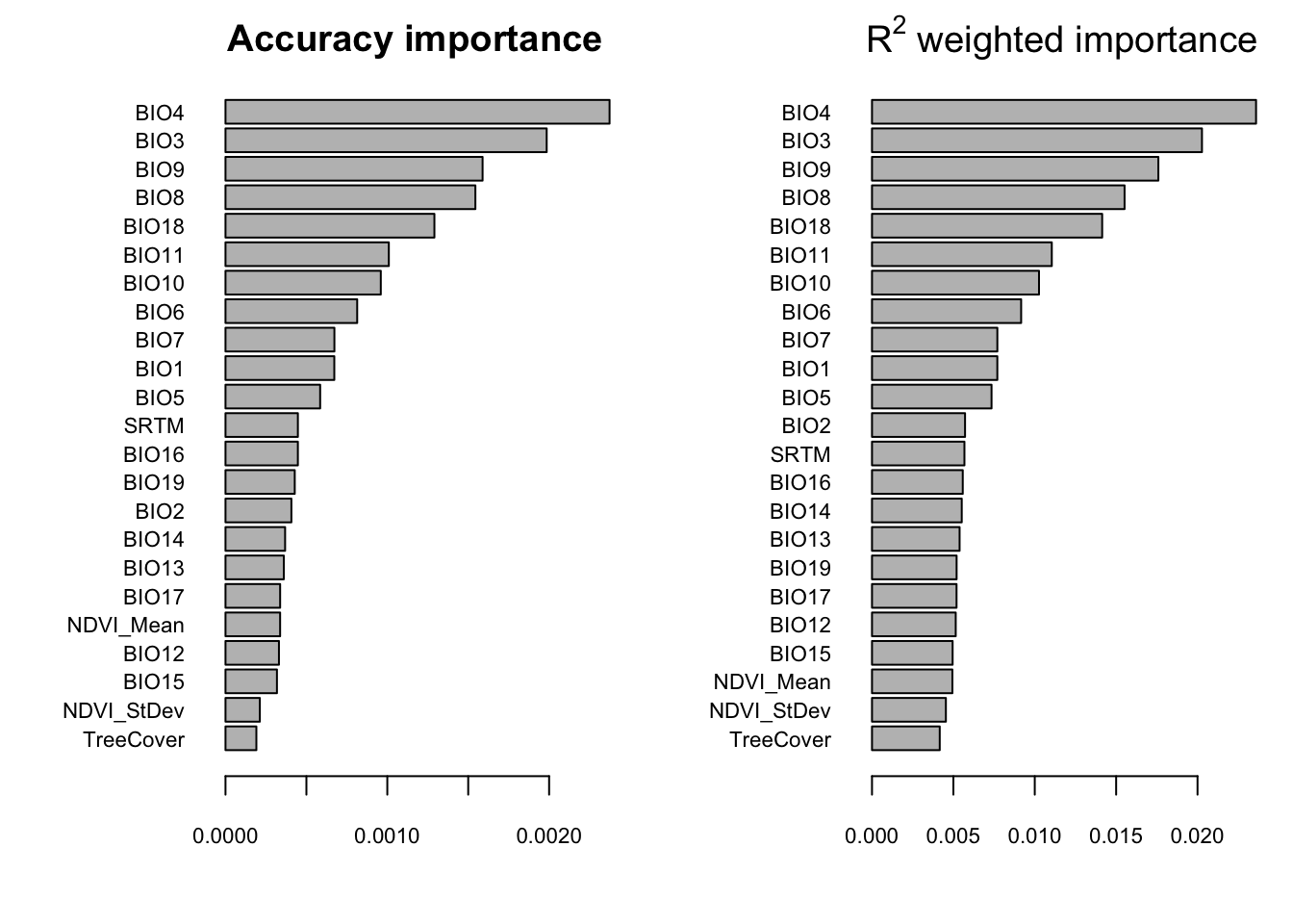

FIGURE 7.2: Overall importance of predictor variables

For the Willow Flycatcher subsetted data in this tutorial, what are the top 5 variables?

Use the code below to look at Cuumulative importance, aka which variants are strongly associated with the top two variables. The cumulative importance is plotted separately for all species and averaged over all species. The cumulative importance can be interpreted as a mapping from an environmental gradient on to biological gradient.

plot(wiflforest,plot.type="Cumulative.Importance")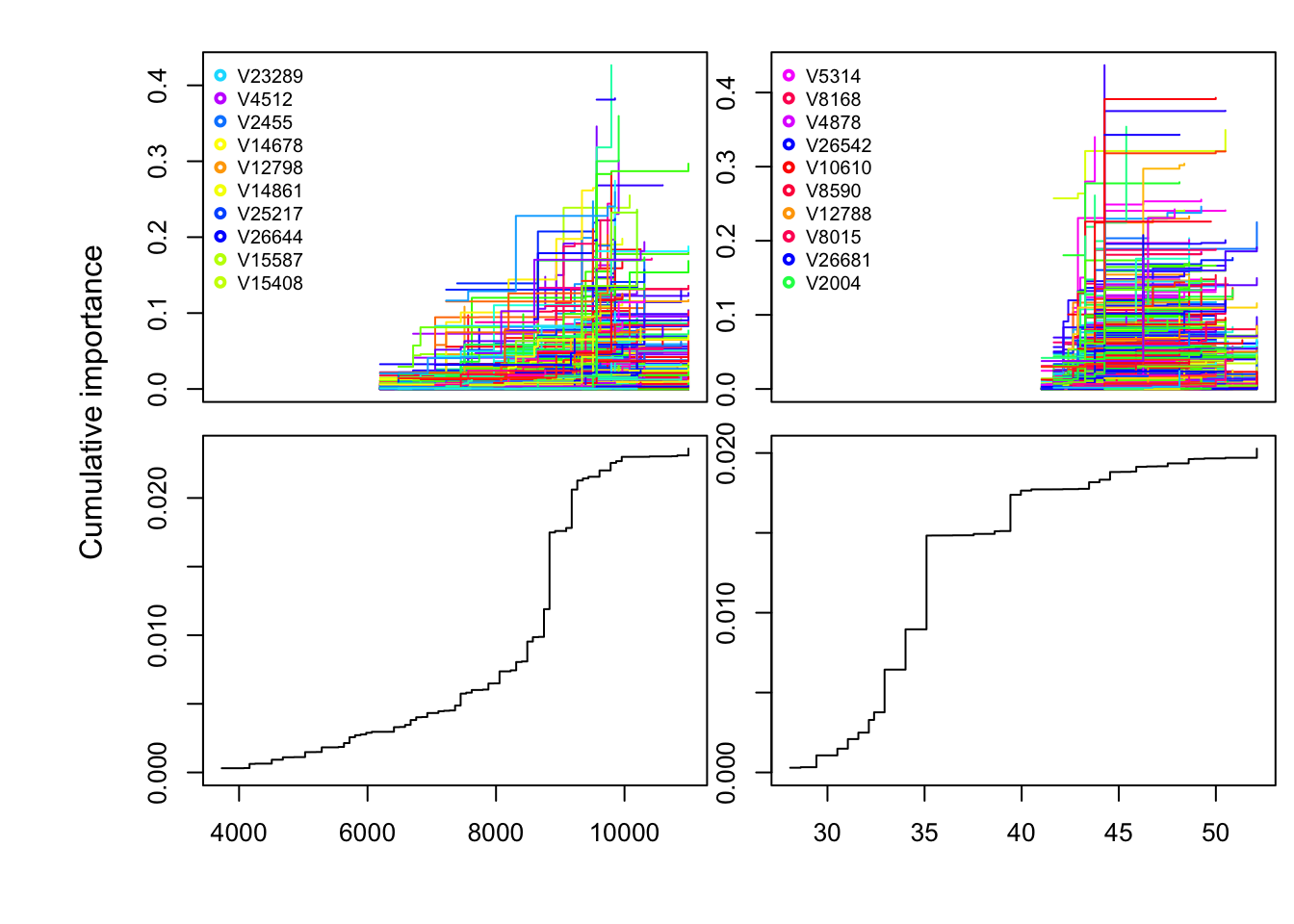

FIGURE 7.3: Individual and cumulative importance of SNPs associated with top 2 environmental variables

Which SNP has the greatest importance? For plotting purposes, only the first two top environmental variables are plotted. So the plots on the left are variants and turnover functions associated with Bio4, and the plots on the right are associated Bio3.

You can confirm this by looking at the range of your top environemntal variables and comparing it to the x-axis in the plots above using this code below:

Ewifl %>% dplyr::select(BIO4,BIO3) %>% summarise(rangeBio4=range(BIO4),rangeBio3=range(BIO3))

## # A tibble: 2 × 2
##   rangeBio4 rangeBio3
##       <dbl>     <dbl>
## 1      3298        27
## 2     11946        54

#or 

Ewifl %>% pull(BIO4) %>% range()

## [1]  3298 11946

Ewifl %>% pull(BIO3) %>% range()

## [1] 27 54

Note, while gradient forest can look at variants associated with environmental variables like this, we tend to choose the top uncorrelated environmental variables and run latent factor mixed models to identify candidate genes associated with each environmental variable. Why? In gradient forest, we “bin” the variation, so we are looking for large patterns, not individual variants.

7.5 Basic Gradient Forest Preparation

So now that you see how gradient forest is run, let’s plot the results in space.

Gradientforest here was based off of 21 locations in the WIFL range. I’ve randomly chosen 100,000 points within the WIFL range and gotten the evironmental data for these 100,000 sites, which will allow us to have a more continuous view of important environmental associations in WIFL space. Load your 100,000 random points with associated environmental predictors. This can be created with another script that was included with the tutorial material (bioclim&randoms.R), but we’ll use the ready-made grid created specifically for Willow Flycatchers.

#WIFL current random points, filter out 'bad' points
birdgrid<- read_csv("data/6.0/wiflcurrentRH.csv") %>% #load your  random points with assocaited env predictors
  filter(BIO4!="-9999") %>%  #remove the "bad data"
  as.data.frame() #create the data frame

## Rows: 100000 Columns: 12

## ── Column specification ───────────────────────────────
## Delimiter: ","
## dbl (12): X, Y, BIO2, BIO3, BIO4, BIO5, BIO8, BIO9,...

## 
## ℹ Use `spec()` to retrieve the full column specification for this data.
## ℹ Specify the column types or set `show_col_types = FALSE` to quiet this message.

##Let's look at bird grid, untransformed environmental variable
head(birdgrid)

##         X     Y BIO2 BIO3 BIO4 BIO5 BIO8 BIO9 BIO11
## 1  -76.17 44.09  103   26 9755  260   93   -5   -60
## 2 -103.38 42.94  164   36 9842  320  183  -43   -43
## 3  -69.11 44.32  113   29 9282  261   28  187   -54
## 4 -109.13 33.49  197   52 6719  287  175  121     9
## 5 -106.01 33.40  169   46 7305  314  214   84    37
## 6 -119.89 48.97  102   32 7206  167  -92   52   -98
##   BIO15 BIO17 BIO18
## 1    14   201   224
## 2    64    32   167
## 3    14   256   256
## 4    60    47   200
## 5    65    42   156
## 6    25   105   117

dim(birdgrid)

## [1] 99541    12

We don’t have to use all the predictors in the next steps, in this case, we’ll use the top 4 uncorrelated variables. These variables were selected by moving down the list of ranked importance for the full model and discarding variables highly correlated (|Pearson’s r| > 0.7) with a variable of higher importance. You can see the correlations among environmental variables across your sample sites. While it is clearly hard to read here, if you export this and open in excel, you can color code and keep track of the correlations among the ranked variables.

head(cor(Ewifl,method="pearson"))

##          BIO1     BIO2     BIO3    BIO4     BIO5
## BIO1  1.00000  0.06378  0.41991 -0.3227  0.70423
## BIO2  0.06378  1.00000  0.20607  0.2063  0.51230
## BIO3  0.41991  0.20607  1.00000 -0.8978 -0.07301
## BIO4 -0.32265  0.20626 -0.89779  1.0000  0.33424
## BIO5  0.70423  0.51230 -0.07301  0.3342  1.00000
## BIO6  0.81738 -0.18653  0.73399 -0.7881  0.22968
##         BIO6    BIO7     BIO8    BIO9    BIO10   BIO11
## BIO1  0.8174 -0.3214  0.41036  0.6098  0.83681  0.8838
## BIO2 -0.1865  0.4967 -0.07870  0.2901  0.21572 -0.0240
## BIO3  0.7340 -0.7323 -0.33935  0.7733 -0.07723  0.7565
## BIO4 -0.7881  0.9472  0.39863 -0.6709  0.24630 -0.7257
## BIO5  0.2297  0.4142  0.46587  0.3243  0.92631  0.3598
## BIO6  1.0000 -0.7907  0.02865  0.7580  0.37954  0.9787
##         BIO12     BIO13   BIO14    BIO15    BIO16
## BIO1 -0.06788 -0.009306 -0.3315  0.47177 -0.01376
## BIO2 -0.62811 -0.527137 -0.5750  0.03587 -0.54400
## BIO3  0.11332  0.283245 -0.4859  0.62916  0.27646
## BIO4 -0.43212 -0.542562  0.1622 -0.52172 -0.54341
## BIO5 -0.49614 -0.468213 -0.4053  0.10623 -0.47815
## BIO6  0.29580  0.381466 -0.2247  0.56762  0.38053
##        BIO17   BIO18    BIO19 NDVI_Mean NDVI_StDev
## BIO1 -0.3092 -0.3012  0.05711  -0.25183    -0.3159
## BIO2 -0.6153 -0.3973 -0.50485  -0.71683    -0.5122
## BIO3 -0.4319 -0.6322  0.38306  -0.12471    -0.3679
## BIO4  0.0850  0.4621 -0.64819  -0.19234     0.1161
## BIO5 -0.4351 -0.2278 -0.43996  -0.57552    -0.3845
## BIO6 -0.1567 -0.4205  0.48703   0.03524    -0.1907
##          SRTM TreeCover
## BIO1 -0.55867  -0.22919
## BIO2  0.62444  -0.31430
## BIO3  0.04009   0.04665
## BIO4  0.17262  -0.19766
## BIO5 -0.19354  -0.41770
## BIO6 -0.54098   0.01015

For the remaining time in this tutorial we are focusing on the uncorrelated variables determined for the full Willow Flycatcher dataset (Ruegg et al. 2017), BIO11 (Mean temperature of coldest quarter), BIO5 (Max temperature of warmest month), BIO4 (Temperature seasonality (standard deviation *100)), and BIO17 (Precipitation of driest quarter).

Predict across your random sites using your Forest model:

predictors_uncor<-c("BIO11","BIO5","BIO4" ,"BIO17")

currentgrid <-cbind(birdgrid[,c("X","Y")], predict(wiflforest,birdgrid[,predictors_uncor])) #predict across your random sites using your forest

##Let's look at currentgrid, transformed environmental variables
##Notice how they were transformed
head(currentgrid)

##         X     Y      BIO11      BIO5     BIO4
## 1  -76.17 44.09  0.0004528  0.001014 0.022466
## 2 -103.38 42.94  0.0013002  0.002946 0.022643
## 3  -69.11 44.32  0.0005108  0.001068 0.021303
## 4 -109.13 33.49  0.0050652  0.002272 0.003932
## 5 -106.01 33.40  0.0064085  0.002934 0.004638
## 6 -119.89 48.97 -0.0001678 -0.002423 0.004499
##       BIO17
## 1 0.0049102
## 2 0.0007953
## 3 0.0057301
## 4 0.0014202
## 5 0.0013088
## 6 0.0025174

dim(currentgrid)

## [1] 99541     6

We can summarize the variation using principal components. We then convert those PC axes to RGB values for plotting.

#Getting the PCs and Converting Them to RGB Color Values
PCs=prcomp(currentgrid[,3:6]) #run your PCs on your top four variables
# set up a colour palette for the mapping
a1 <- PCs$x[,1]
a2 <- PCs$x[,2]
a3 <- PCs$x[,3]
r <- a1+a2
g <- -a2
b <- a3+a2-a1
r <- (r-min(r)) / (max(r)-min(r)) * 255
g <- (g-min(g)) / (max(g)-min(g)) * 255
b <- (b-min(b)) / (max(b)-min(b)) * 255
wiflcols=rgb(r,g,b,max=255)
wiflcols2=col2rgb(wiflcols)
wiflcols3=t(wiflcols2)
gradients=cbind(currentgrid[c("X","Y")],wiflcols3)

The multi-dimensional biological space can be plotted by taking the principle component of the transformed grid and presenting the first two dimensions in a biplot. You’ve already defined the PCs above and the RGB color palette. Different coordinate positions in the biplot represent differing allele frequency compositions as associated with the predictors.

##Biplot specifics
nvs <- dim(PCs$rotation)[1]
vec <- c("BIO11","BIO5","BIO4" ,"BIO17")
lv <- length(vec)
vind <- rownames(PCs$rotation) %in% vec
scal <-100
xrng <- range(PCs$x[, 1], PCs$rotation[, 1]/scal) *1.2
yrng <- range(PCs$x[, 2], PCs$rotation[, 2]/scal) *1.2
plot((PCs$x[, 1:2]), xlim = xrng, ylim = yrng, pch = ".", cex = 4, col = rgb(r, g, b, max = 255), asp = 1)
points(PCs$rotation[!vind, 1:2]/scal, pch = "+")
arrows(rep(0, lv), rep(0, lv), PCs$rotation[vec,1]/scal, PCs$rotation[vec, 2]/scal, length = 0.0625)
jit <- 0.0015
text(PCs$rotation[vec, 1]/scal + jit * sign(PCs$rotation[vec,1]), PCs$rotation[vec, 2]/scal + jit * sign(PCs$rotation[vec,2]), labels = vec)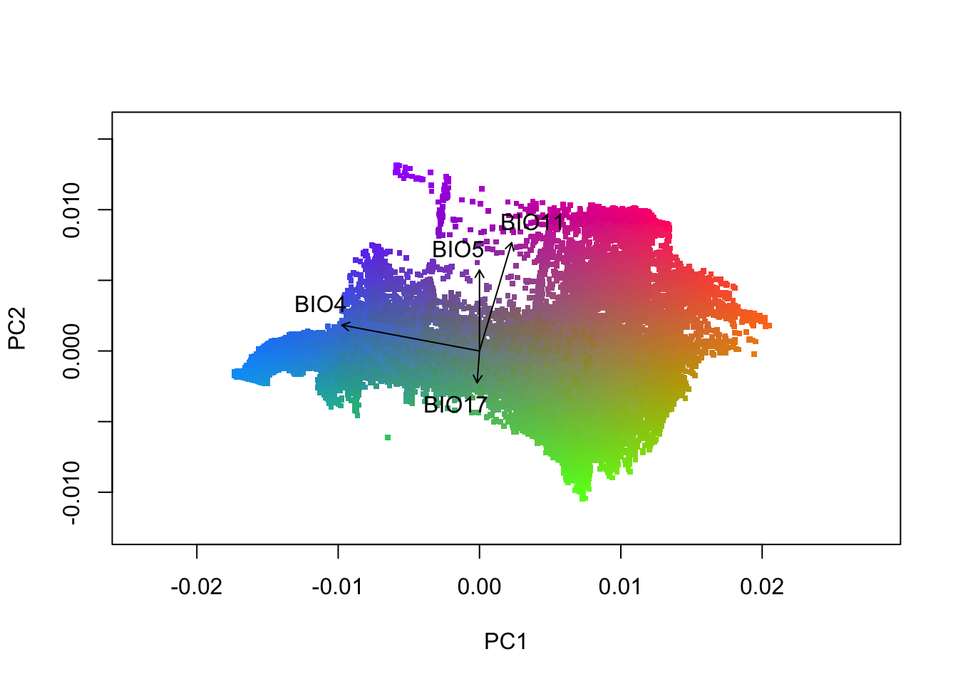

FIGURE 7.4: A principle component plot of the top 4 uncorrelated variables

Save this image using the code chunk below. What environmental variables are associated with the colors green, pink and blue? Knowing this will help with the interpretation of plotting this in space.

dir.create("stored_results/6.0", showWarnings = FALSE, recursive = TRUE)
pdf("stored_results/6.0/WIFL.PCA_uncorrelated.pdf")
nvs <- dim(PCs$rotation)[1]
vec <- c("BIO11","BIO5","BIO4" ,"BIO17")
lv <- length(vec)
vind <- rownames(PCs$rotation) %in% vec
scal <-100
xrng <- range(PCs$x[, 1], PCs$rotation[, 1]/scal) *1.2
yrng <- range(PCs$x[, 2], PCs$rotation[, 2]/scal) *1.2
plot((PCs$x[, 1:2]), xlim = xrng, ylim = yrng, pch = ".", cex = 4, col = rgb(r, g, b, max = 255), asp = 1)
points(PCs$rotation[!vind, 1:2]/scal, pch = "+")
arrows(rep(0, lv), rep(0, lv), PCs$rotation[vec,1]/scal, PCs$rotation[vec, 2]/scal, length = 0.0625)
jit <- 0.0015
text(PCs$rotation[vec, 1]/scal + jit * sign(PCs$rotation[vec,1]), PCs$rotation[vec, 2]/scal + jit * sign(PCs$rotation[vec,2]), labels = vec)
dev.off()

## quartz_off_screen 
##                 2

With this, we can draw our first gradient forest map:

wiflcols <- rgb(r,g,b,max=255)
wiflcols2 <- col2rgb(wiflcols)
wiflcols3<- t(wiflcols2)
gradients<-cbind(currentgrid[c("X","Y")],wiflcols3)
wiflmap<-gradients
coordinates(wiflmap)<- ~X+Y #setting the coordinates
proj4string(wiflmap) <- CRS("+proj=longlat +datum=WGS84")

par(mar=c(0,0,0,0))
plot(wiflmap,col=rgb(r,g,b,max=255),pch=15)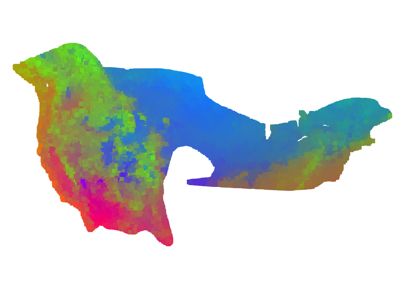

FIGURE 7.5: Our gradient forest model of SNP variation in the Willow Flycatcher breeding range

How would you interpret the different colors on thie WIFL map? Is the endangered southwest Willow Flycatcher locally adapted?

Let’s plot this another way, on an actual map of North America. To do this, we need some additional shapefiles.

The domain here allows you to crop the shapefiles to just your species range.

library(sf)
coastlines <- st_read("data/6.0/ne_shapefiles/ne_10m_coastline.shp")

## Reading layer `ne_10m_coastline' from data source 
##   `/Users/eriq/Documents/git-repos/merida-workshop-2022/data/6.0/ne_shapefiles/ne_10m_coastline.shp' 
##   using driver `ESRI Shapefile'
## Simple feature collection with 4133 features and 3 fields
## Geometry type: LINESTRING
## Dimension:     XY
## Bounding box:  xmin: -180 ymin: -85.22 xmax: 180 ymax: 83.63
## Geodetic CRS:  WGS 84

domain <- c(
  xmin = -140, 
  xmax = -55,
  ymin = 15,
  ymax = 50
)

coast_cropped <- st_crop(coastlines, domain)

## Warning: attribute variables are assumed to be
## spatially constant throughout all geometries

This code allows you to plot, but also change the domain to what will encompass your species shapefile. Suffice it to say I went through a fair number of iterations to ge it right.

Once you have the shapefiles and cropped domain, you can create a map, project the map, and then crop it to what region you want. Using the above code, the domain can/should be larger than what you will be plotting. You can further crop later!

library(ggspatial)
countries_cropped <-  st_read("data/6.0/ne_shapefiles/ne_10m_admin_0_boundary_lines_land.shp") %>%
  st_crop(domain)

## Reading layer `ne_10m_admin_0_boundary_lines_land' from data source `/Users/eriq/Documents/git-repos/merida-workshop-2022/data/6.0/ne_shapefiles/ne_10m_admin_0_boundary_lines_land.shp' 
##   using driver `ESRI Shapefile'
## Simple feature collection with 462 features and 18 fields
## Geometry type: MULTILINESTRING
## Dimension:     XY
## Bounding box:  xmin: -141 ymin: -55.12 xmax: 141 ymax: 70.08
## Geodetic CRS:  WGS 84

## Warning: attribute variables are assumed to be
## spatially constant throughout all geometries

states_cropped <- st_read("data/6.0/ne_shapefiles/ne_10m_admin_1_states_provinces_lines.shp") %>%
  st_crop(domain)

## Reading layer `ne_10m_admin_1_states_provinces_lines' from data source `/Users/eriq/Documents/git-repos/merida-workshop-2022/data/6.0/ne_shapefiles/ne_10m_admin_1_states_provinces_lines.shp' 
##   using driver `ESRI Shapefile'
## Simple feature collection with 10114 features and 21 fields
## Geometry type: MULTILINESTRING
## Dimension:     XY
## Bounding box:  xmin: -178.1 ymin: -49.25 xmax: 178.4 ymax: 81.13
## Geodetic CRS:  WGS 84

## Warning: attribute variables are assumed to be
## spatially constant throughout all geometries

mapg <- ggplot() +
  geom_sf(data = coast_cropped) +
  geom_sf(data = countries_cropped, fill = NA) +
  geom_sf(data = states_cropped, fill = NA) +
  ggspatial::layer_spatial(wiflmap,col=rgb(r,g,b,max=255),pch=15) +
  geom_sf(data=wifl_shape,fill=NA) +
  theme_bw() 

mapg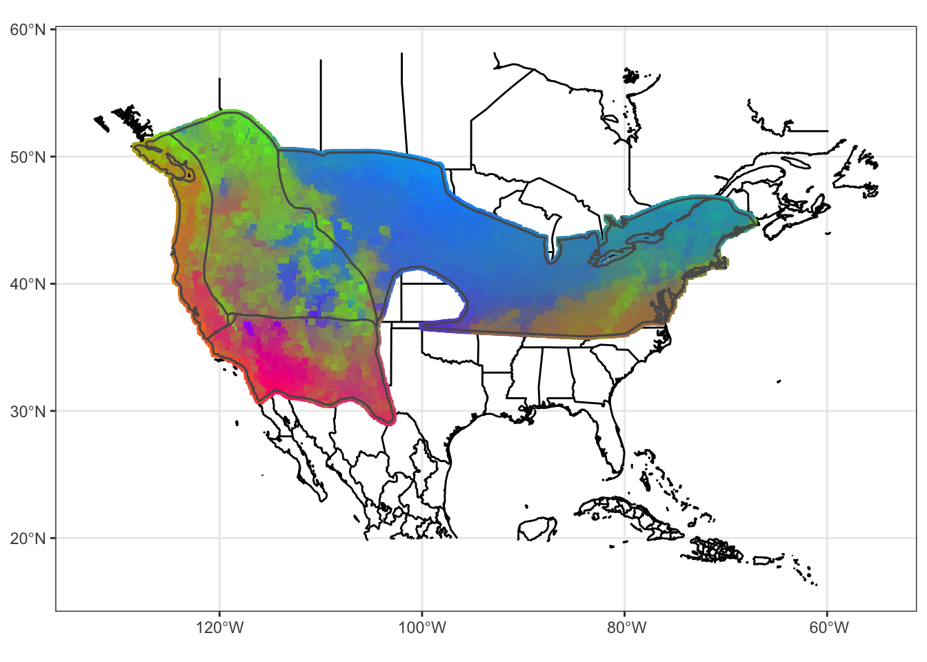

FIGURE 7.6: Our gradient forest model of SNP variation in the Willow Flycatcher breeding range on a map

Now, let’s see how our developing map looks under such a projection. We just define lamproj as a coordinate reference system and pass it in to coord_sf()

lamproj <- "+proj=lcc +lat_1=20 +lat_2=60 +lat_0=40 +lon_0=-100 +x_0=0 +y_0=0 +ellps=GRS80 +datum=NAD83 +units=m +no_defs"

#Plotting with projection, and cutting out rectangle (Don't need a lot of extra space)
rectangled <-mapg +
  xlab("Longitude") + ylab("Latitude")+
  coord_sf(
    crs = st_crs(lamproj), 
    xlim = c(-2200476.8, 2859510), 
    ylim = c(-1899797, 1809910.8),
    expand = FALSE) 
rectangled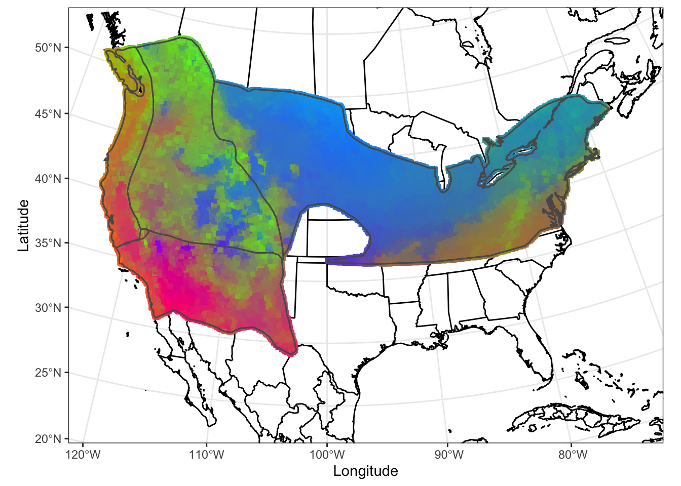

Rename this file. I put the plot I plotted in here, but let’s make sure this works for you!!

ggsave("stored_results/6.0/WIFL.GF_map.pdf")

## Saving 7 x 5 in image

7.6 Defining “Genomic Vulnerability/Genomic offset” Given Future Climate Predictions

The plots above are the genotype-environment relationship given present-day climate rasters. However, we know rapid fluctuations in temperature and precipitation associated with climate change can alter the suitability of particular regions making it necessary for individuals to either adapt, disperse or die if the changes are extreme enough. Those species that possess standing genetic variation for climate-related traits (i.e. have adaptive capacity) are most likely to have the ability to adapt to rapidly changing environments. Those species that unable to adapt are deemed most vulneraable.

To investigate which populations might be most vulnerable to future climate change, we defined the metric “genomic vulnerability” as the mismatch between current and predicted future genomic variation based on genotype-environment relationships modeled across contemporary populations. We followed the method presented in Fitzpatrick and Keller (2015) to calculate genomic vulnerability using an extension of the gradient forest analysis. Populations with the greatest mismatch are least likely to adapt quickly enough to track future climate shifts, potentially resulting in population declines or extirpations.

Here, we read in the future climate predictions for each random point. Since different amounts of heat-trapping gases released into the atmosphere by human activities produce different projected increases in Earth’s temperature, we provided two such predicted models: the 2.6 emission predictions and the 8.5 emission predictions for the year 2050.

The lowest recent emissions pathway (RCP), 2.6, assumes immediate and rapid reductions in emissions and would result in about 2.5°F of warming in this century. The highest emissions pathway, RCP 8.5, roughly similar to a continuation of the current path of global emissions increases, is projected to lead to more than 8°F warming by 2100, with a high-end possibility of more than 11°F. Each of these is a composite of multiple prediction models and have rather different predictions.

future1<-read_csv("data/6.0/wiflfuture2-6-2050.csv") %>% 
  filter(BIO4!="-9999") %>% 
  as.data.frame()

## Rows: 100000 Columns: 12

## ── Column specification ───────────────────────────────
## Delimiter: ","
## dbl (12): X, Y, BIO2, BIO3, BIO4, BIO5, BIO8, BIO9,...

## 
## ℹ Use `spec()` to retrieve the full column specification for this data.
## ℹ Specify the column types or set `show_col_types = FALSE` to quiet this message.

head(future1)

##         X     Y BIO2 BIO3 BIO4 BIO5 BIO8 BIO9 BIO11
## 1  -76.17 44.09  102   26 9584  283   65  138   -34
## 2 -103.38 42.94  166   36 9942  342  171  -15   -24
## 3  -69.11 44.32  112   29 9209  282   42  173   -31
## 4 -109.13 33.49  202   51 6941  310  195  133    24
## 5 -106.01 33.40  174   46 7508  338  235  109    53
## 6 -119.89 48.97  101   31 7244  192  -70   82   -79
##   BIO15 BIO17 BIO18
## 1    16   209   221
## 2    63    35   155
## 3    17   259   273
## 4    69    33   202
## 5    71    30   153
## 6    33    97   107

future2<-read_csv("data/6.0/wiflfuture8-5-2050.csv") %>% 
  filter(BIO4!="-9999") %>% 
  as.data.frame()

## Rows: 100000 Columns: 12

## ── Column specification ───────────────────────────────
## Delimiter: ","
## dbl (12): X, Y, BIO2, BIO3, BIO4, BIO5, BIO8, BIO9,...

## 
## ℹ Use `spec()` to retrieve the full column specification for this data.
## ℹ Specify the column types or set `show_col_types = FALSE` to quiet this message.

head(future2)

##         X     Y BIO2 BIO3  BIO4 BIO5 BIO8 BIO9 BIO11
## 1  -76.17 44.09  101   26  9652  299   46  175   -19
## 2 -103.38 42.94  166   35 10238  359  183   -6   -15
## 3  -69.11 44.32  111   29  9211  295   45  209   -18
## 4 -109.13 33.49  203   51  7078  323  208  142    33
## 5 -106.01 33.40  175   45  7602  351  249  127    63
## 6 -119.89 48.97  101   30  7521  210  -64  111   -70
##   BIO15 BIO17 BIO18
## 1    16   215   224
## 2    62    41   153
## 3    19   257   269
## 4    69    30   198
## 5    75    27   152
## 6    37    87    90

We then use our gradient forest model to transform these into “biological space” just as we did for random points across contemporary environments.

futuregrid <- cbind(future1[,c("X","Y")], predict(wiflforest,future1[,predictors_uncor]))

Finally, we calculate genomic vulnerability. Mathematically, for a given point this is the Euclidean distance between the current biological space (currentgrid) and the future biological space (futuregrid):

coords<-birdgrid[,c("X","Y")]
euc <- matrix(data=NA,nrow=nrow(futuregrid),ncol=3)
for(j in 1:nrow(currentgrid)) {
  euc[j,] <- c(as.numeric(coords[j,]), 
               as.numeric(dist(rbind(currentgrid[j,], futuregrid[j,]))))
}

euc <- data.frame(euc)
names(euc) <- c("Long","Lat","Vulnerability")
head(euc)

##      Long   Lat Vulnerability
## 1  -76.17 44.09      0.001783
## 2 -103.38 42.94      0.001586
## 3  -69.11 44.32      0.001739
## 4 -109.13 33.49      0.001362
## 5 -106.01 33.40      0.002192
## 6 -119.89 48.97      0.001132

This again takes a moment. Once we have this metric, we can easily map genomic vulnerability across the range. First by choosing a color palette, then by converting a dataframe of distances to a spatial polygon and giving it the same extent as the map it’s going to be plotted on and finally, mapping in ggplot.

library(scales)
colramp2=rev(brewer.pal(n = 9, name = "RdYlBu")[c(1:9)])
Futcolors<-colorRampPalette(colramp2)
show_col(Futcolors(100))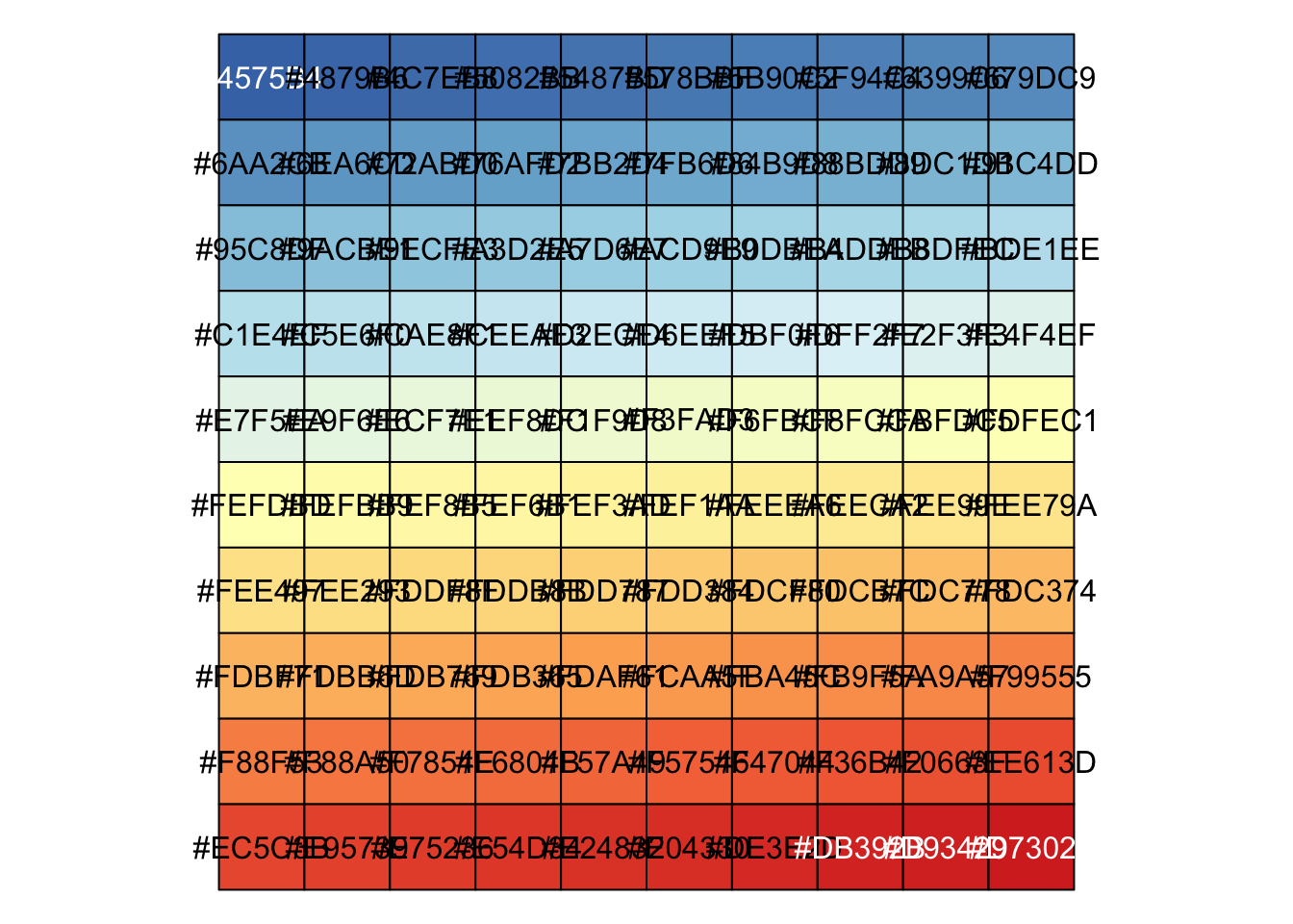

FIGURE 7.7: Color Ramp for plotting

Notice that in the rev in the above code chunk will reverse the RColorBrewer color palette so the highest vulnerablity corresponds to the red color, rather than blue.

euc_sp<-st_as_sf(euc,coords=c("Long", "Lat"))
st_crs(euc_sp) <- st_crs(coast_cropped) 

mapg <- ggplot() +
  geom_sf(data = coast_cropped) +
  geom_sf(data = countries_cropped, fill = NA) +
  geom_sf(data = states_cropped, fill = NA) +
  geom_point(data=euc,aes(x=Long,y=Lat,color=Vulnerability),pch=15,size=.5) +
  scale_colour_gradientn(colours = Futcolors(100)) +
   geom_sf(data=wifl_shape,fill=NA) +
  theme_bw() 

mapg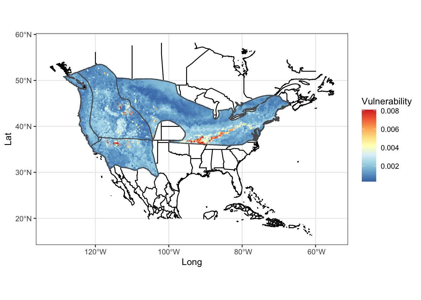

FIGURE 7.8: Heat map of genomic vulnerability under the 2050 2.6 emission future prediction

How does this look if we plot the second scenario of higher gas emissions? Compare and contrast the two scenarios, keeping in mind that the colors are scaled within each scenario.

futuregrid2 <- cbind(future2[,c("X","Y")], predict(wiflforest,future2[,predictors_uncor]))

coords<-birdgrid[,c("X","Y")]
euc2 <- matrix(data=NA,nrow=nrow(futuregrid2),ncol=3)
for(j in 1:nrow(currentgrid)) {
  euc2[j,] <- c(as.numeric(coords[j,]), 
                as.numeric(dist(rbind(currentgrid[j,], futuregrid2[j,]))))
}
euc2 <- data.frame(euc2)
names(euc2) <- c("Long","Lat","Vulnerability")

euc_sp2<-st_as_sf(euc2,coords=c("Long", "Lat"))
st_crs(euc_sp2) <- st_crs(coast_cropped) 

mapg2 <- ggplot() +
  geom_sf(data = coast_cropped) +
  geom_sf(data = countries_cropped, fill = NA) +
  geom_sf(data = states_cropped, fill = NA) +
  geom_point(data=euc2,aes(x=Long,y=Lat,color=Vulnerability), pch=15,size=0.5) +
  scale_colour_gradientn(colours = Futcolors(100))+
  geom_sf(data=wifl_shape,fill=NA) +
  theme_bw() 

mapg2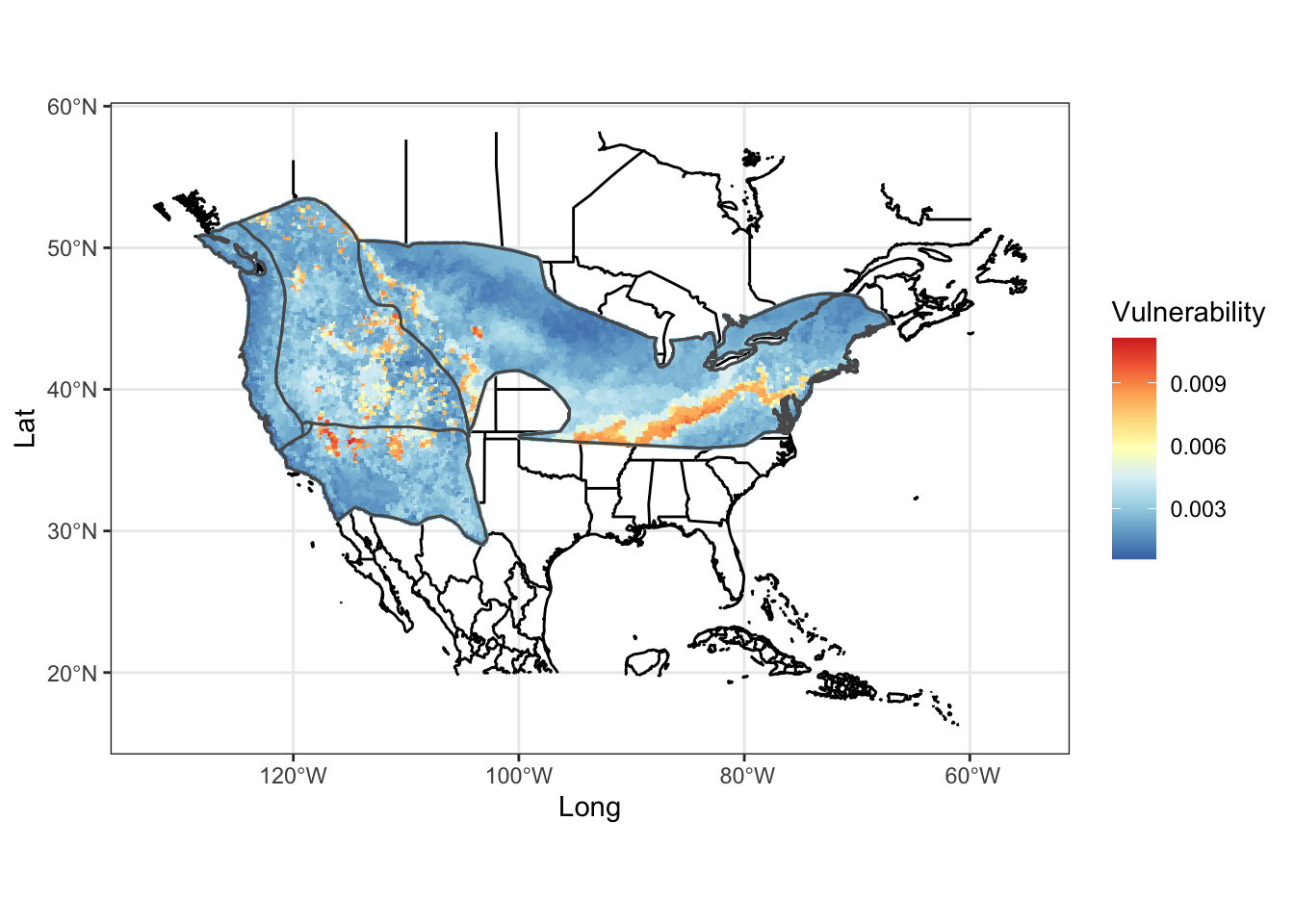

FIGURE 7.9: Heat map of genomic vulnerability under the 2050 8.5 emission future prediction

7.7 Next steps

7.7.1 Randomization

So as we’ve seen in this tutorial, grandient forest is a great way to understand which variables are important drivers of the population genomic structure of your species and with plotting the assoiciations in space, a great way to look at local adpation of different populations to different environmental variables. To understand how important, whether local adaptation is significant in your species, you need to run a randomization step. In this step, you are breaking up the actual associations of allele frequencies and enviornmnetal variables, randomizing the environmental predictors and running gradient forest again multiple times.

This code below is not evaluated because it takes a very long time to run one thousand randomizations.

realtotal=wiflforest$species.pos.rsq
realaverage=sum(wiflforest$result)/realtotal
realaverage

for (i in 1:1000){

predsR=Ewifl[sample(nrow(Ewifl)),]

wiflforestR=gradientForest(cbind(predsR,Gwifl), predictor.vars=colnames(predsR), response.vars=colnames(Gwifl), ntree=10, transform = NULL, compact=F, maxLevel=1,trace=F,nbin=101)

 randtotal=wiflforestR$species.pos.rsq
 randaverage=sum(wiflforestR$result)/randtotal

 #totaldiff=realtotal-randtotal
 #avrdiff=realaverage-randaverage

 write.table(randtotal,file=paste("stored_results/6.0/WIFL.randtotal",sep=""),row.names=FALSE,col.names=FALSE,append=T)
 write.table(randaverage,file=paste("stored_results/6.0/WIFL.randaverage",sep=""),row.names=FALSE,col.names=FALSE,append=T)
}

randa <- read_delim("stored_results/6.0/WIFL.randaverage",delim="\t",col_names = F)
randt=read.table("stored_results/6.0/WIFL.randtotal",delim="\t", col.names = F)
quantile(randa$V1,c(0.975))
#randa=as.numeric(randa)
#randt=as.numeric(randt)

library(ggpubr)
pdf("wiflforest.1000regtrees.hist.pdf")
par(mfrow=c(2,1))
hist(randa$V1,xlim=c(0.001,0.5), main="Average R-squared of Random Gradient Forests",xlab="Average R-squared of 10,000 WIFL SNPs")
abline(v=0.2006884,col="red") #replace with the 95th percential of the average R squared from real data
dev.off()

If your real results fall right in the middle of the randomized results, then even though you have ranked environmental variables underlying the population structure of your species, it’s no different than random, and therefore not significant.

7.7.2 Candidate variants

If you find that gradient forest is significant, your next step might be wanting to identify variants associated with these top variables. Grandient forest is not really the way to do this. Rather, there are two programs that you can use: Latent Factor Mixed Models (LFMM) and Redundancy Analyses (RDA).

• LFMM can identify candidate loci associated with top ranking environmental variables

https://bcm-uga.github.io/lfmm/

• RDA is a method to extract and summarise the variation in a set of response variables that can be explained by a set of explanatory variables. More accurately, RDA is a direct gradient analysis technique which summarises linear relationships between components of response variables that are “redundant” with (i.e. “explained” by) a set of explanatory variables. Very similar to gradient forest, but also can identify candidate genes associated with environmental variables.

https://popgen.nescent.org/2018-03-27_RDA_GEA.html