Session 5 Finding and Obtaining Environmental Data for Conservation

This is an introduction to environmental layers for conservation genomics analysis, which was created for the UCMexus Conservation Genomics Workshop 2022. This overview covers coordinate systems, projections, raster data and various examples of commonly-used environmental layers.

5.1 Environmental Layers. A general overview

This section provides a brief narrative of Marius Someveille’s PowerPoint presentation. We are trying to succinctly capture the main points in this web/bookdown version so that it might easily be translated with Google Translate.

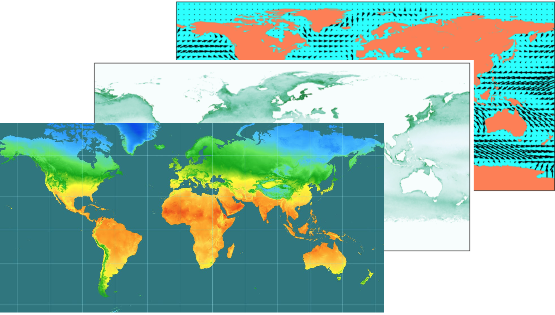
Environmental layers in this context are raster data they carry information about particular “cells” or “pixels” of the earth’s surface. All of these terms will be defined in detail later. For now, here are a few pictures of what environmental layers might look like when they are plotted and displayed:

5.1.1 Environmental layers in conservation genetics

5.1.1.1 Landscape connectivity analysis (gene flow)

Connectivity is essential for long term persistence of populations and metapopulations as it affects gene flow. Functional connectivity is the degree to which individuals move through a landscape, which is affected by landscape features and environmental heterogeneity. Landscape genetics tests which landscape and environmental factors best explain genetic connectivity among populations and highlights which landscape features need to be maintained or enhanced to facilitate connectivity (gene flow) for different species.

For example, Robertson et al. (2018) studied frogs in multiple locations in North America, shown here:

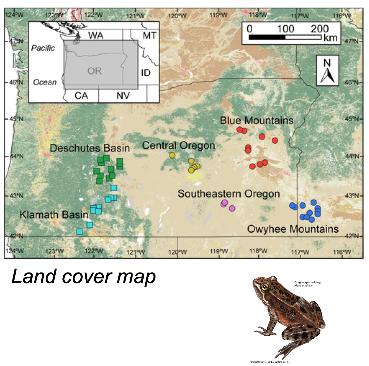
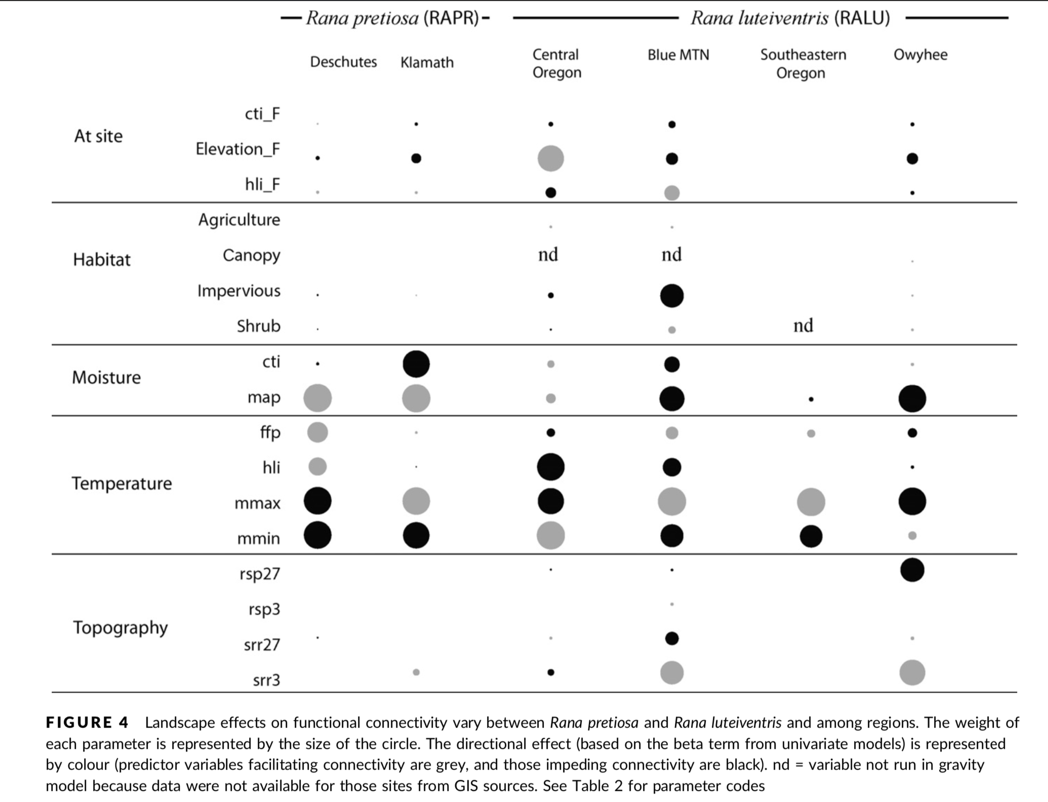
The positions of samples are shown here on a map that was created from land cover data. However, many other layers area available, giving information of, for example, topography, temperature, and moisture levels in the different locations. Landscape genetics approaches were used to identify which of these features were most associated with connectivity between populations in each of the different regions (i.e, different colors on the map). They summarized those results as follows:

5.1.1.2 Environmental Niche Analysis

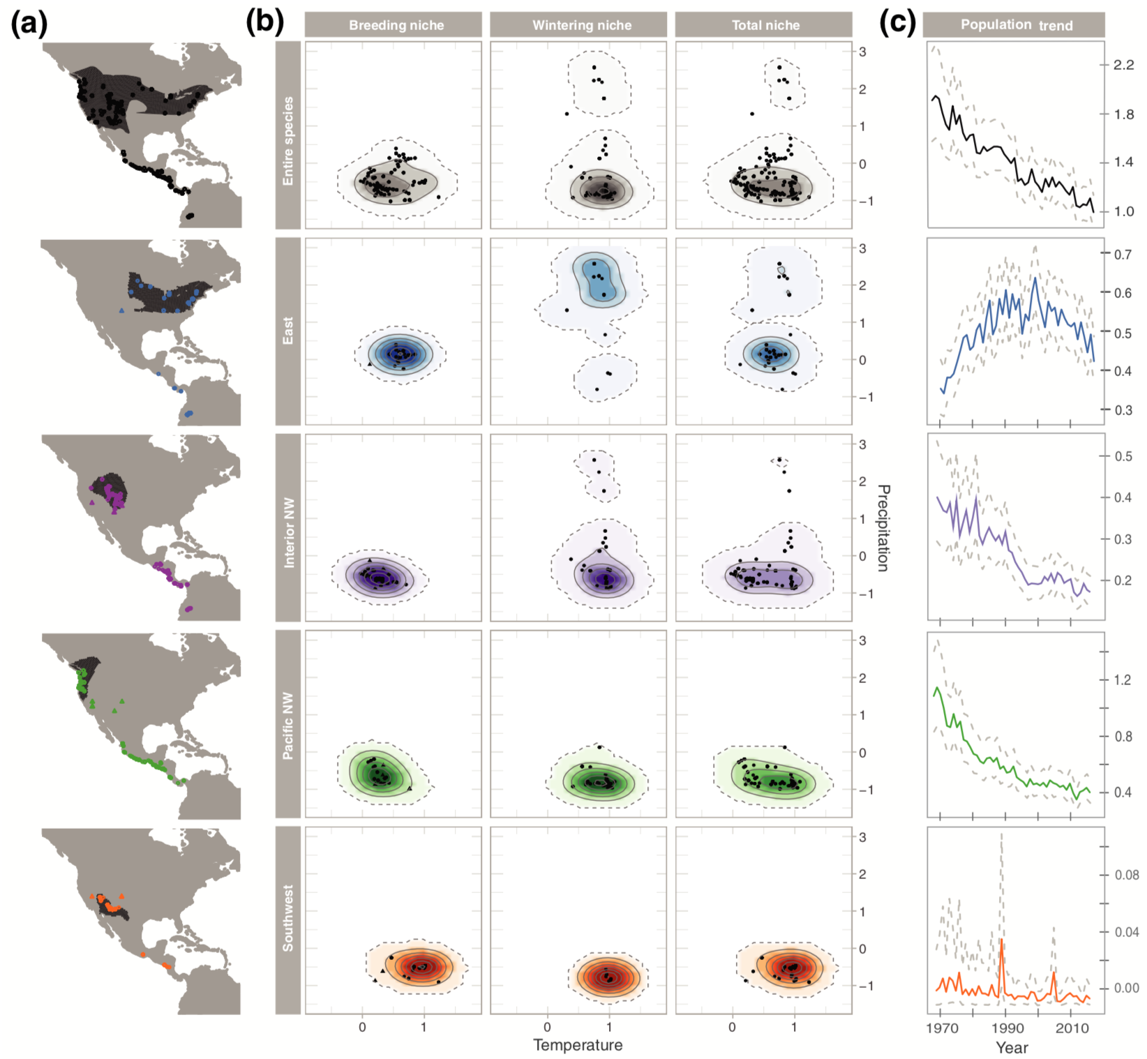
Ruegg et al. (2021) shows another example of the use of environmental layers in conservation genetics. In this case, genetic differences resolved separate breeding populations of the Willow Flycatcher, Empidonax traillii, in North America, and also made it possible to identify where birds from each breeding population spend their winters, as shown in the following figure (in which the different breeding populations are denoted by different colors):

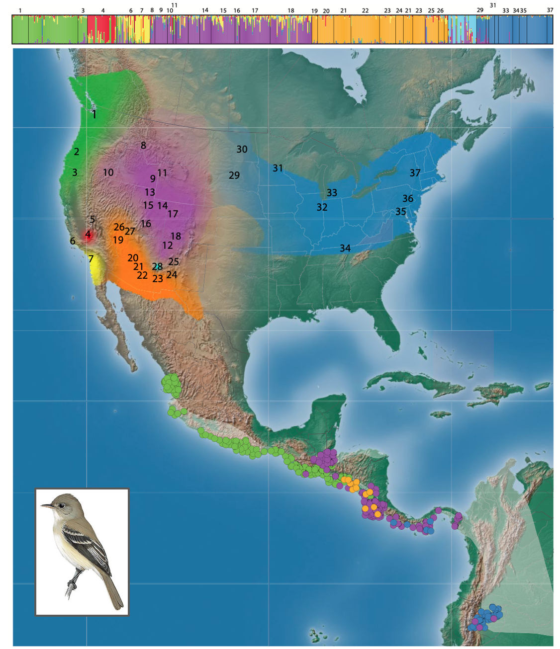
With the breeding and wintering areas for each subpopulation identified, climate layers (temperature and precipitation) were used to identify the climatic conditions that defined the birds breeding and wintering niches for the subpopulations. Population trends were found to be associated with overlap between breeding and wintering niches, with the subpopulation showing the least niche overlap being the only subpopulation not showing a decreasing trend.

5.1.1.3 Genome-environment association to study vulnerability

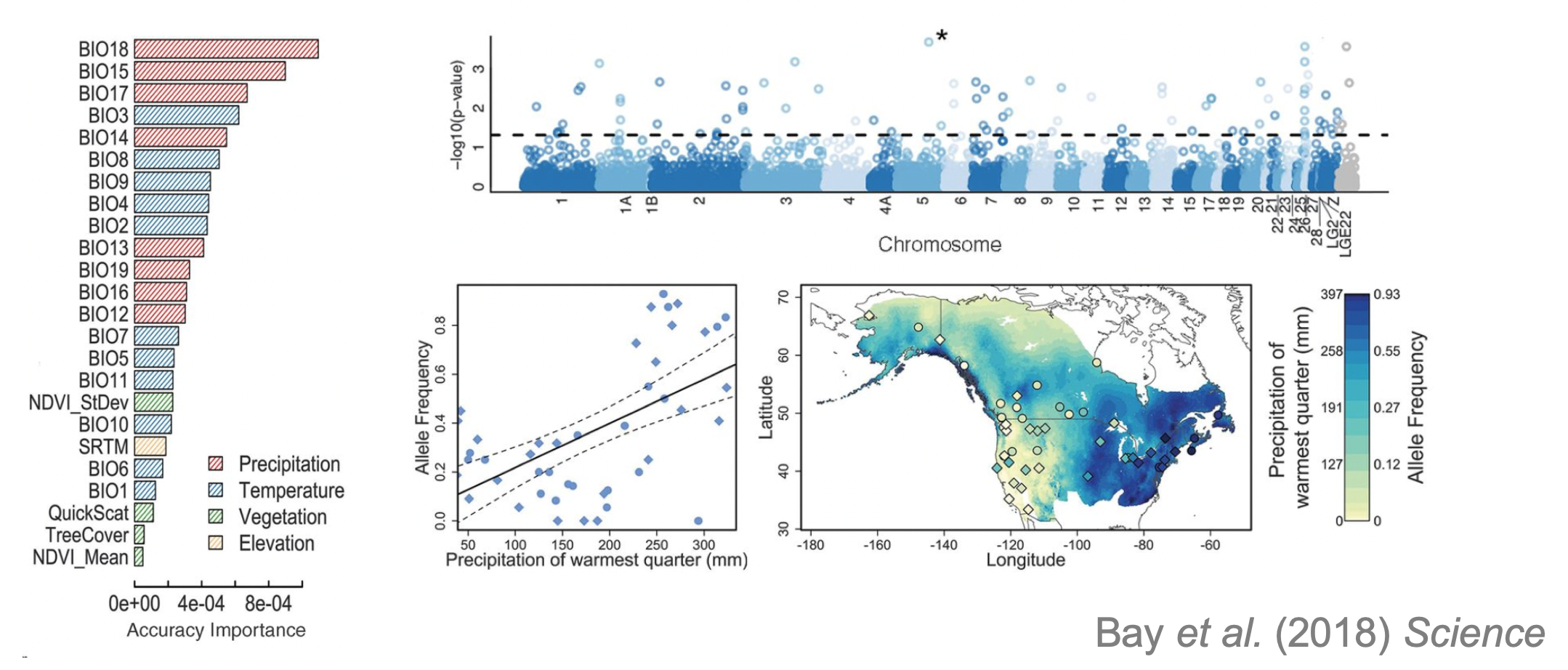
Associations between genetic variation and environmental variation (that we will hear about from Christen Bossu!) can be used to identify places where there is expected to be a mismatch between expected genetic patterns and environmental conditions after changes due to climate change. One of the first papers documenting this was Bay et al. (2018).

In their study, a variety of environmental predictors (BIO18, BIO15, etc.), whose values across space are represented by environmental layer data, were found to be associated with genetic variation, as shown in the following montage of figures from the paper:

5.1.1.4 Environmental layers as raster data

Digital environmental layers are obtained by abstracting reality in either vector or raster format, as shown below:

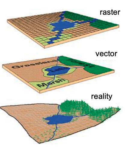
The most common format encountered for environmental layers is raster, which is composed of a grid of cells like this:

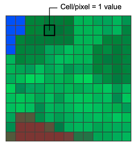
A cell value can represent a measured value at the center point of the cell (e.g. elevation) or for the whole cell square (average, max, category). The cell values represent the phenomenon portrayed by the raster dataset such as a category (e.g. grassland, forest, road), magnitude (e.g. noise pollution, rainfall), height (e.g. elevation), or spectral value. Cell values can be either positive or negative, integer, or floating point.

Commonly used format to store rasters on a computer are: TIFF, Hierarchichal Data Format (HDF), JPEG, NetCDF.

5.1.1.5 Coordinate system and projections

For geographic analysis, we use a coordinate system that uses a three-dimensional spherical surface to determine location on the Earth. Each point on Earth is defined by a latitude value and a longitude value, which are measures of angle as shown in the following figure:

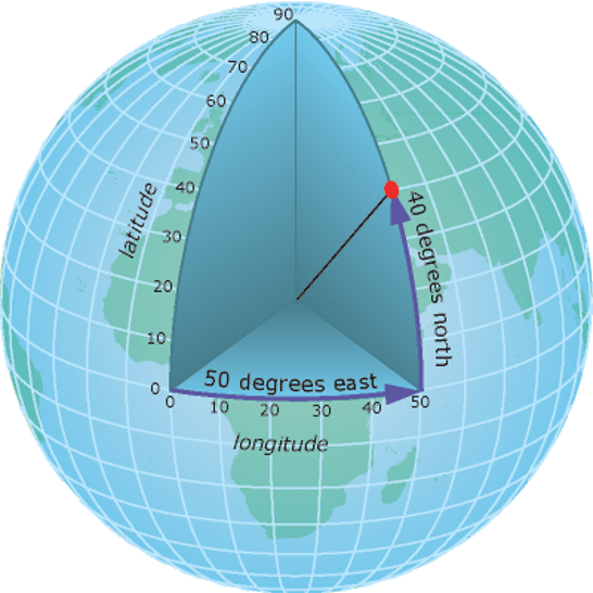
The units of the geographic coordinate system are units of angle as follows: 1 degree = 60 arc-minutes = 3600 arc-seconds.

To visualize geographic data as maps, we need to draw it on a two-dimensional surface using a projected coordinate system. Map projections tell how to distort the earth so that it is displayed on a flat surface. A coordinate reference system (CRS) then defines how the projected map is related to real places on the earth. Many projections exist, here are some examples:

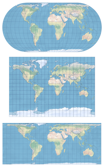
Good practice: raster data storing environmental layers should have a projection, and choose one projection for the whole analysis, i.e. converting all of the geographic data into the same projection.

5.1.1.6 Parameters of raster data

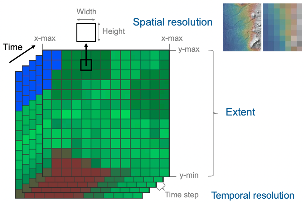
Rasters storing environmental layers are defined by multiple parameters. The extent is defined by the top, bottom, left, and right coordinates of the rectangular area covered by a raster. The spatial resolution is defined by the width and height of cells/pixels (cells are square and the width and height of all cells have the same value), usually given in degree / arc-minute / arc-second. For environmental variables that have layers at different time, it is possible to stack these layers and define a temporal extent. i.e. the first and last date, and temporal resolution, which is the time step (e.g. daily, weekly, monthly, yearly).

5.1.1.7 Examples of climate layers

Source	Method	Variables	Extent	Spatial resolution	Temporal resolution
WorldClim	Interpolation of observations from weather stations	Temperature Precipitation Solar radiation BIOCLIM	Global	30 sec (~1km2) 2.5 min 5 min 10 min (~340 km2)	Monthly 1970 – 2000
Chelsa	Quasi-mechanistical downscale of global circulation model	Temperature Precipitation BIOCLIM	Global	30 arc sec (~1km2)	Monthly 1979 – 2018
Prism	Statistical model using weather station data and atmospheric process	Temperature Precipitation	USA	30 arc sec (~1km2)	Monthly 1981–2010

5.1.2 Examples of atmospheric layers

Source	Method	Variables	Extent	Spatial resolution	Temporal resolution
NOAA Global Forecast System	Global atmospheric model	Wind direction Wind speed	Global	0.5 deg	6 times / day 2011 – present
WorldClim	Interpolation of observations from weather stations	Wind speed Water vapor pressure	Global	30 sec (~1km2) 2.5 min 5 min 10 min (~340 km2)	Monthly 1970 – 2000

5.1.3 Examples of vegetation layers

Source	Method	Variables	Extent	Spatial resolution	Temporal resolution
VIP30 (NASA)	Remote sensing using spectrometer on board satellites	NDVI EVI	Global	0.05 deg ~5.6km	Monthly 1981 – 2014
Copernicus (ESA)	Remote sensing using spectrometer on board satellites	NDVI EVI	Global	300m	10-day Present
GEDI (NASA)	Remote sensing using lidar (laser ranging) onboard the ISS	Vertical profile of vegetation: canopy height, canopy vertical structure, ground elevation	51.6 deg N and S latitudes	25m	Annual Present

5.1.4 Examples of landscape layers

Source	Method	Variables	Extent	Spatial resolution	Temporal resolution
SRTM (NASA)	Remote sensing using radar onboard satellites	Elevation	Global	1 arc-second (~30m)	NA
MODIS (NASA)	Remote sensing using spectrometer onboard satellites	Snow cover	Global	30 arc-sec (~1km2)
Copernicus (ESA)	remote sensing + random forest for classification	Land cover	Global	100m	NA
NASA Gridded Population of the World	Input data are census tables	Human population density	Global	30 arc-sec (~1km2)	NA 2000–2020

References

Bay RA, Harrigan RJ, Le Underwood V et al. (2018) Genomic signals of selection predict climate-driven population declines in a migratory bird. Science, 359, 83–86.

Robertson JM, Murphy MA, Pearl CA et al. (2018) Regional variation in drivers of connectivity for two frog species (rana pretiosa and r. Luteiventris) from the US pacific northwest. Molecular ecology, 27, 3242–3256.

Ruegg K, Anderson EC, Somveille M et al. (2021) Linking climate niches across seasons to assess population vulnerability in a migratory bird. Global Change Biology.