population-growth-with-spip • CKMRpop

library(CKMRpop)

The default simulation engine for CKMRpop, spip, is not well suited to scenarios with population growth or other size changes. This is because the survival rates cannot be set to vary over time. So the only way that population growth or decline occurs is by manipulating the number of individuals entering the population each year.

This is done with the --cohort-size parameter. Specifically, if you are doing a simulation for T years, you can do like this:

--cohort-size var J1 J2...JT

where J1 … JT are T integers giving the number of individuals entering the population each year. As the spip documentation says:

        this makes the expected cohort size each year from
        MaxAge to T+MaxAge-1 equal to J1 J2...JT respectively. Hence there
        must be T such arguments J following the var option (where T is the
        number of years that the simulation will run---the argument to the -T
        or the --number-of-years option.)

The CKMRpop function leslie_from_spip() provides a way to figure out what the initial number of individuals should be, and what the cohort sizes should be each year to simulate a growing or shrinking population that has reached an equilibrium stable age distribution. (I suspect that few populations of interest actually reach this type of equilibrium—certainly not fish populations with high recruitment variability—but for some purposes it will be important to be able to simulate such a population.)

Note that this is only implemented correctly for scenarios in which male and female age-specific survival rates are the same.

Here we demonstrate how to simulate with population growth and decline in that equilibrium context.

Starting with a cohort size of 300 at just before the initial time step, we show how to create a 1% rate of increase in the species_1_life_history population for 100 years, and we also show a scenario with a 0.05% rate of decline for 100 years. We can calculate the parameters for both from a single call to leslie_from_spip().

library(CKMRpop)

pars <- leslie_from_spip(
  P = species_1_life_history, 
  C = 300, 
  growth_rates = c(0.01, -0.005), 
  T = 100
)

That object pars has the parameters we need to simulate the population under those scenarios. For the scenarios with specified growth rates, the results we need are in:

pars$growth_rate_results$[["0.01"]]

and

pars$growth_rate_results$[["-0.005"]]

respectively.

Population growth of 0.01

We just have to set up the iniital pop sizes and cohort sizes.

GrowthPars <- species_1_life_history

# always put the number of years in first:
GrowthPars$`number-of-years` <- 100


GrowthPars$`initial-females` <- floor(pars$growth_rate_results$`0.01`$stable_age_distro_fem)
GrowthPars$`initial-males` <- floor(pars$growth_rate_results$`0.01`$stable_age_distro_male)
GrowthPars$`cohort-size` <- pars$growth_rate_results$`0.01`$cohort_size_param_string


# we also add some sampling parameters here
samp_frac <- 0.03
samp_start_year <- 50
samp_stop_year <- 75
GrowthPars$`discard-all` <- 0
GrowthPars$`gtyp-ppn-fem-post` <- paste(
  samp_start_year, "-", samp_stop_year, " ", 
  samp_frac, " ", samp_frac, " ", samp_frac, " ",
  paste(rep(0, GrowthPars$`max-age` - 3), collapse = " "),
  sep = ""
)
GrowthPars$`gtyp-ppn-male-post` <- GrowthPars$`gtyp-ppn-fem-post`

Then we can run the population:

set.seed(5)  # set a seed for reproducibility of results
spip_dir <- run_spip(pars = GrowthPars)  # run spip
slurped <- slurp_spip(spip_dir, 2) # read the spip output into R

Now, let’s plot the population sizes to see it is doing what we expect it to be doing:

ggplot_census_by_year_age_sex(slurped$census_postkill)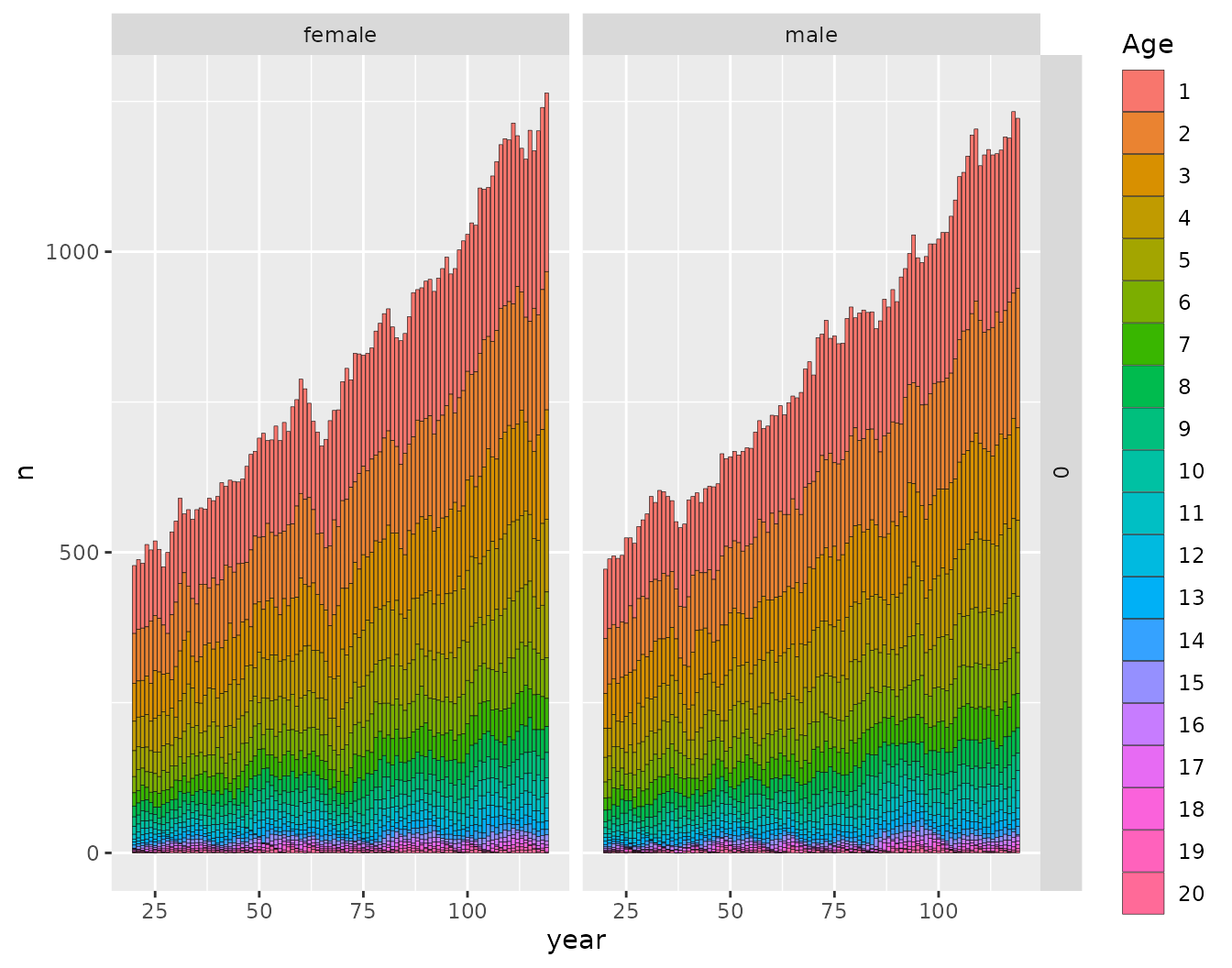

OK, that looks pretty much like it ought to.

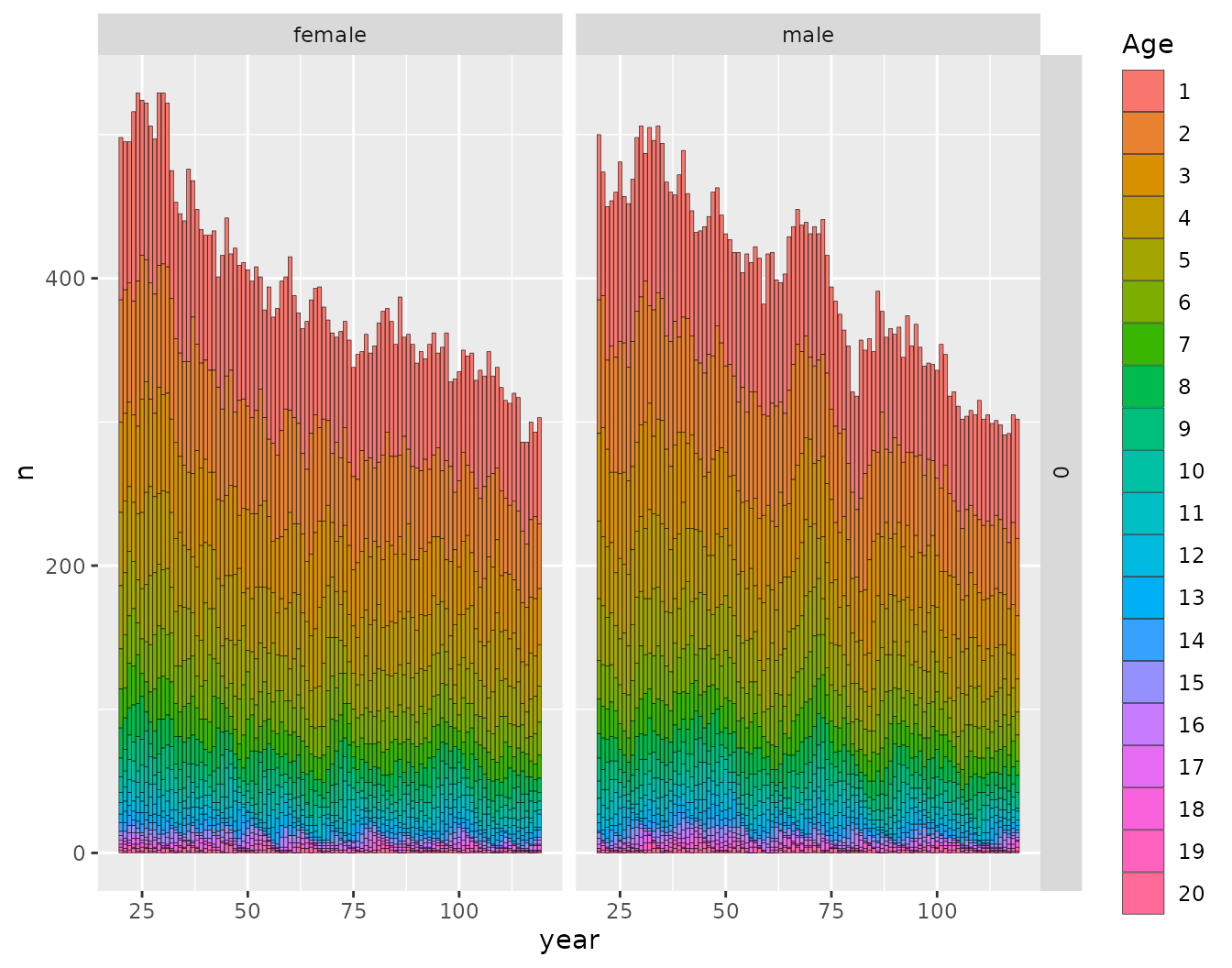
Population decline of 0.005

We just have to set up the iniital pop sizes and cohort sizes.

DeclinePars <- species_1_life_history

# always put the number of years in first:
DeclinePars$`number-of-years` <- 100


DeclinePars$`initial-females` <- floor(pars$growth_rate_results$`-0.005`$stable_age_distro_fem)
DeclinePars$`initial-males` <- floor(pars$growth_rate_results$`-0.005`$stable_age_distro_male)
DeclinePars$`cohort-size` <- pars$growth_rate_results$`-0.005`$cohort_size_param_string


# we also add some sampling parameters here
samp_frac <- 0.03
samp_start_year <- 50
samp_stop_year <- 75
DeclinePars$`discard-all` <- 0
DeclinePars$`gtyp-ppn-fem-post` <- paste(
  samp_start_year, "-", samp_stop_year, " ", 
  samp_frac, " ", samp_frac, " ", samp_frac, " ",
  paste(rep(0, DeclinePars$`max-age` - 3), collapse = " "),
  sep = ""
)
DeclinePars$`gtyp-ppn-male-post` <- DeclinePars$`gtyp-ppn-fem-post`

Then we can run the population:

set.seed(5)  # set a seed for reproducibility of results
spip_dir <- run_spip(pars = DeclinePars)  # run spip
slurped <- slurp_spip(spip_dir, 2) # read the spip output into R

Now, let’s plot the population sizes to see it is doing what we expect it to be doing:

ggplot_census_by_year_age_sex(slurped$census_postkill)