Solving ODEs in R

22 January 2015

Marc Mangel is offering a course in Quantitative Fisheries at NMFS’ Southwest Fisheries Science Center (where I work). Having spent the fall delivering a course about using R to my NMFS colleagues, I thought it would be fun to sit in on Marc’s class. What a great opportunity! I just think it is the coolest thing that Marc is part of our community, and is willing to provide this enjoyable and useful education for us!

Most of my forays into statistical methodology and the mathematics behind them have involved discrete math—I work on topics in genetics that can mostly be condensed down to thinking about drawing balls out of urns. So, I am not terribly familiar with the sorts of dynamical systems that we will be developing in Marc’s class. To make things worse, a rather depressing fraction of any mathematical agility I might have acquired as a graduate student seems to have departed! No really! When I look back at the derivations in my Master’s thesis I think to myself, “Holy Cow! Did I really know how to do that?”

On the other hand, I feel like I actually have gotten better at computer implementation since my graduate years. Hence, my plan for the exercises for this course are to have a good time implementing them in R (since I’ve been enjoying that language immensely over the last couple of years) and plotting lots of pictures of the results and intermediate steps in the hopes that this will help develop some intuition about these problems (and maybe even reach some of the dusty corners of my mind.) And I figured I would put this up on my blog in case other people in the class wanted to see one way to go about solving the first exercise for the course using R.

It has been a long time since I have solved any differential equations, but there is apparently a package called deSolve for R that looks like it should make it relatively painless.

Setup

A good reference is the deSolve vignette I strongly recommend giving that a quick read through.

Installing deSolve

Installing deSolve is straightforward:

install.packages("deSolve")

Exercise 1

Assume a logistically growing population has carrying capacity \(K = 10000\), \(r = 0.3\) and has been depleted to level \(N(1) = 150\). To investigate the recovery strategy, let \(C_{max}(N)\) be the maximum catch that can be taken from the population to sustain it at current level \(N\) and define recovery time to be the first time that population size crosses 6,000.

Compute the recovery time if your harvest strategy is to close the fishery entirely until recovery occurs (i.e. harvest is 0) or harvest is \(0.1 C_{max}(N(t))\), \(0.2 C_{max}(N(t))\), \(\ldots\), \(0.9 C_{max}(N(t))\).

Make a plot of recovery time vs. the fraction of the sustaining catch your strategy allows and think about the social and institutional consequences of these results.

Solution

All of this could be done analytically, but I want to play around with deSolve so let’s just be silly about it and pretend we don’t know the solution to the logistic.

Well, it seems that \(C_{max}(N(t))\) must be whatever value will leave \(\frac{dN}{dt} = 0\), so it is just going to be \(rN(1-N/K)\). Therefore we can easily compute a Logistic function that has a parameter fract.of.max, which we will call fom for short:

library(deSolve)
parameters <- c(r = 0.3, K = 10000, fom = 0)
state <- c(N = 150)
Logistic <- function(t, state, parameters) {
  with(as.list(c(state, parameters)), {
    # rate of change 
    dN <- (1 - fom) * (r * N * (1 - N / K))
    
    # return the result
    list(dN)
  }) # end with(as.list ...
}

times <- seq(0, 300, by = 0.2)

Now we can run that over a range of values of fom:

fracts <- seq(0, 0.9, by = 0.1)
names(fracts) <- paste("frac =", fracts)

list_results <- lapply(fracts, function(x) {
  parameters["fom"] <- x
  ode(y = state, times = times, func = Logistic, parms = parameters)
})

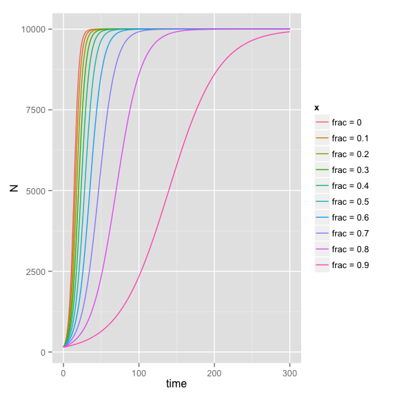
Now we can make a long format data frame out of those and then plot with ggplot

# make a long data frame of it
ldf <- do.call(rbind, lapply(names(list_results), function(x) data.frame(list_results[[x]], x, stringsAsFactors = FALSE)))

# plot with ggplot
library(ggplot2)
ggplot(data = ldf, aes(x = time, y = N, color = x)) + geom_line()

plot of chunk unnamed-chunk-5

Now, to get the times when you first cross 6,000 we can use dplyr (just for fun):

library(dplyr)
ldf <- tbl_df(ldf)

recov_times <- ldf %>% 
  group_by(x) %>% 
  summarise(recov = min(time[N>6000]))

recov_times

## Source: local data frame [10 x 2]
## 
##             x recov
## 1    frac = 0  15.4
## 2  frac = 0.1  17.2
## 3  frac = 0.2  19.2
## 4  frac = 0.3  22.0
## 5  frac = 0.4  25.6
## 6  frac = 0.5  30.8
## 7  frac = 0.6  38.4
## 8  frac = 0.7  51.2
## 9  frac = 0.8  76.6
## 10 frac = 0.9 153.2

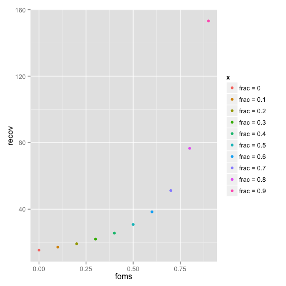
And then we can plot those against the fraction of the sustaining harvest.

# here is some heinous sapply foo to break "frac = 0.1" to a numeric 0.1, etc....
recov_times$foms <- as.numeric(sapply(strsplit(recov_times$x, " = "), "[", 2))

ggplot(recov_times, aes(x = foms, y = recov, color = x)) + geom_point()

plot of chunk unnamed-chunk-7

But it seems that what is really interesting is the total harvest over that time.

Late, and running out of steam…maybe more later. At least I hope this gives a sense for how to use deSolve.