Plotting SST with ggplot

24 December 2014

Roy M and I were curious about how one might go about efficiently and quickly plotting big rasters like sea surface temperature data using ggplot with nice coastlines in there, etc.

I had considered using ggmap. For reasons to do with the mercator projection of the base map in ggmap the word on the street is that this doesn’t work very well. I regularly crashed my whole R session trying it, too! So, instead we will focus on using the GSHHS shoreline maps.

A Catalina Island Example

I am going to be heading out to Catalina Island for some snorkeling with the family over Xmas break. A lot of friends have told me that the water there is warmer than typical this time of year. It seems this would make a good test case. So, here is my plan:

First figure out how to plot this year’s 8-day composite SST for a large area around Catalina Island, using ggplot2.
Then, I want to compare across, say, 9 years, using faceting in ggplot.

Before we get going, here are the libraries that I will be using:

library(stringr)
library(ncdf4)
library(reshape2)
library(ggplot2)
library(mapdata)
library(maptools)

Getting SST data

Roy showed me how to download the data. I am going to wrap that up in a little function that downloads data from Dec 12 in the year that I tell it to, and saves that in an intermediate file, so it doesn’t have to re-download it. Note that, since the other things we will be plotting assume that western hemisphere longitudes are negative, we subtract 360 from the SST longitudes. I also add the date to the output list, as I will want to use that later.

# This is based on code that Roy sent me for getting SST.
# I modified it to get data from around Catalina Island
my_get_sst_catalina <- function(year) {
  # base url with YEAR meant to be replaced
  turl <- "http://coastwatch.pfeg.noaa.gov/erddap/griddap/erdMWsstd8day.nc?sst[(YEAR-12-12T00:00:00Z)][(0.0)][(30.0):(35.0)][(238.0):(243.2)]"
  
  # the URL with YEAR replaced with a value
  the_url <- str_replace(turl, "YEAR", year)
  
  # the filename to save the downloaded data in
  the_file <- paste("sst_", year, ".nc", sep="")
  
  # if the file isn't here, download it
  if(!file.exists(the_file)) {
    download.file(the_url, the_file, mode='wb')
  } else {
    message(paste("Using existing file", the_file, collapse = " "))
  }
  
  # now, grab stuff out of the netcdf file and return it in a list
  # called ret
  sstFile <- nc_open(the_file)
  ret <- list()
  ret$lats <- ncvar_get(sstFile, "latitude")
  ret$lon <- ncvar_get(sstFile, "longitude") - 360 # we need them as negative values
  ret$time <- ncvar_get(sstFile, "time")
  ret$sst <- ncvar_get(sstFile, "sst")
  ret$date <- paste("12-12-", year, sep = "")
  nc_close(sstFile)
  
  ret
}

Here is an example of how to use that function, and a summary of the output.

cata_sst_2014 <- my_get_sst_catalina(2014)

# look at the structure of the result
str(cata_sst_2014)

## List of 5
##  $ lats: num [1:401(1d)] 30 30 30 30 30.1 ...
##  $ lon : num [1:417(1d)] -122 -122 -122 -122 -122 ...
##  $ time: num [1(1d)] 1.42e+09
##  $ sst : num [1:417, 1:401] 19.8 19.9 20 20.2 20.1 ...
##  $ date: chr "12-12-2014"

The sst component is a matrix with elements that correspond to cells of latitude and longitude. It is a raster.

Prepping for ggplot and a simple plot

You might recall that ggplot operates on long-format data frames. A raster in matrix format is in wide format. So, we need to convert that. We can do that pretty easily with the reshape2 package. The trick here is to put the long’s and lat’s on as row and column names and then melt it. I will wrap this up in a function so we can use it easily later. I will also cbind the date to the result, and make a column for Fahrenheit because when most people (in the backwards, non-metric US) are thinking of swimming in cold water, they gauge temp in Fahrenheit (myself included…):

melt_sst <- function(L) {
  dimnames(L$sst) <- list(long = L$lon, lat = L$lats)
  ret <- melt(L$sst, value.name = "sst")
  cbind(date = L$date, ret, degF = ret$sst * 9/5 + 32)
}

And here is how we use that function. And a look at what it returns.

msst <-  melt_sst(cata_sst_2014)
head(msst)

##         date   long lat   sst  degF
## 1 12-12-2014 -122.0  30 19.83 67.69
## 2 12-12-2014 -122.0  30 19.87 67.77
## 3 12-12-2014 -122.0  30 20.00 68.00
## 4 12-12-2014 -122.0  30 20.15 68.28
## 5 12-12-2014 -122.0  30 20.08 68.15
## 6 12-12-2014 -121.9  30 20.09 68.17

Now that we have a long format data frame, we can plot the contents of it with geom_raster in ggplot. (Note that most people think of raster data as being in a matrix format, but, like all things ggplot, geom_raster still requires the data to be in long format).

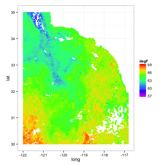
Here is a simple plot:

ggplot(data = msst, aes(x = long, y = lat, fill = degF)) + 
  geom_raster(interpolate = TRUE) +
  scale_fill_gradientn(colours = rev(rainbow(7)), na.value = NA) +
  theme_bw() +
  coord_fixed(1.3)

plot of chunk super-vanilla-sst

That is standard ggplot stuff. Worth mentioning though is coord_fixed which sets the aspect ratio to something that looks good in this part of the world, and the na.value argument to scale_fill_gradientn which ensure that missing data areas don’t get any color on them.

Adding some coastline

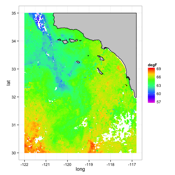
The plot above is sort of nice, but it is ugly to have the coast being the same non-color as missing data, and there is not clean edge on the coast. We will fix that.

A previous post (need to link) showed how to use the GSHHS shoreline maps. We use it here too.

Here we get the data that we need for that. Note that if you want to do this yourself, you would need to download the maps and probably change the path to them below:

if (!rgeosStatus()) gpclibPermit()

# path to the GSHHS maps on my computer
gshhs.f.b <- "/Users/eriq/Maps/gshhg-bin-2.3.3/gshhs_f.b"
shore <- getRgshhsMap(gshhs.f.b, xlim = c(-122, -116.8), ylim = c(30, 35))

## Data are polygon data
## Data are polygon data
## Rgshhs: clipping 2 of 22 polygons ...

shore <- fortify(shore)

The fortify() command turns the polygons from the GSHHS maps into a long data format that ggplot can deal with. Here is what shore looks like now:

head(shore)

##     long   lat order  hole piece group id
## 1 -116.8 31.98     1 FALSE     1   2.1  2
## 2 -116.8 31.98     2 FALSE     1   2.1  2
## 3 -116.8 31.98     3 FALSE     1   2.1  2
## 4 -116.8 31.98     4 FALSE     1   2.1  2
## 5 -116.8 31.98     5 FALSE     1   2.1  2
## 6 -116.8 31.98     6 FALSE     1   2.1  2

Now, adding that coastline in there is as simple as just laying down the polygons in another layer. We give it a gray fill and a black coastline.

basic_plot <- ggplot(data = msst, aes(x = long, y = lat, fill = degF)) + 
  geom_raster(interpolate = TRUE) +
  geom_polygon(data = shore, aes(x=long, y = lat, group = group), color = "black", fill = "grey80") +
  scale_fill_gradientn(colours = rev(rainbow(7)), na.value = NA) +
  theme_bw() +
  coord_fixed(1.3)

basic_plot

plot of chunk basic-plot-with-shore

Harnessing the power of ggplot

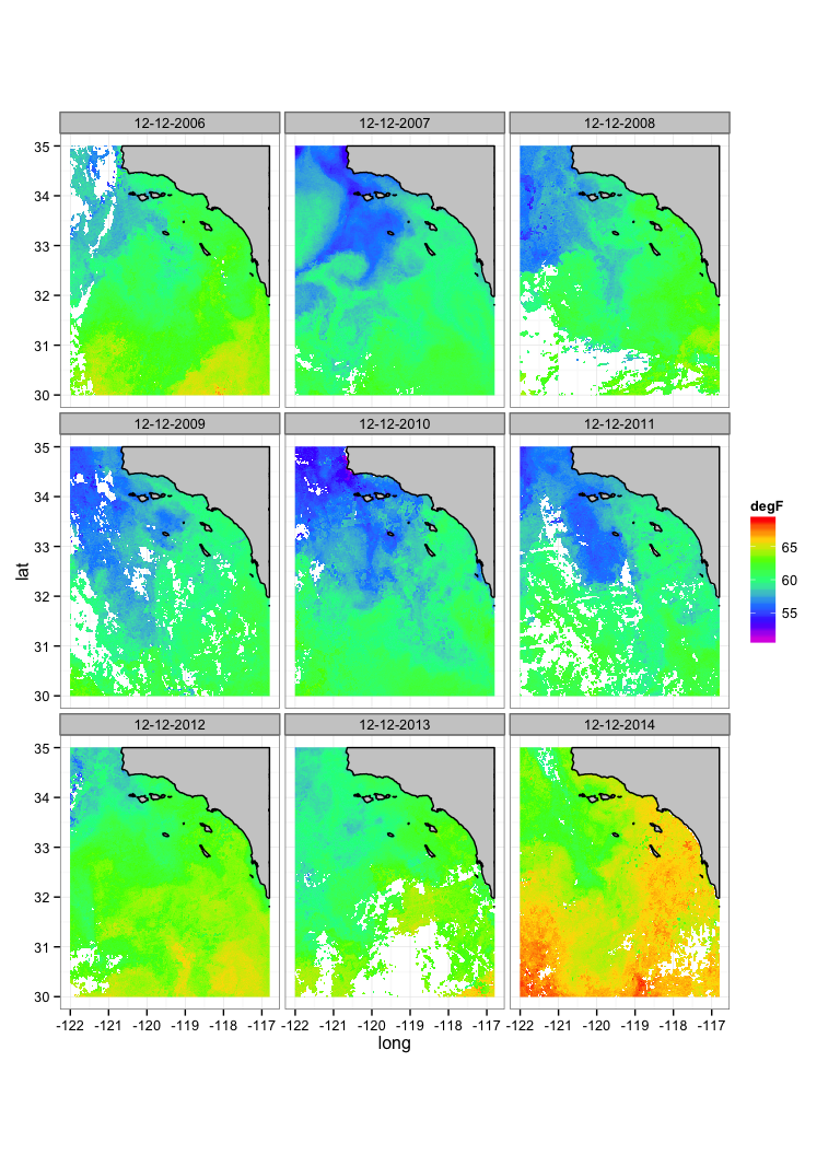
The above is pretty, but recall that I want to compare temperatures on Dec 12 this year, to temps in the 8 previous years. One of the lovely things about using ggplot to plot our sea surface temperatures is that we have immediate access to all of ggplot’s features like faceting.

So, let’s do this. First we have to download all the data for 2006-2014 and put it all together into a single data frame. Like so:

years <- 2006:2014
tmp <- lapply(years, function(x) melt_sst(my_get_sst_catalina(x)))
allyears <- do.call(rbind, tmp)

# see what that looks like:
head(allyears)

##         date   long lat   sst  degF
## 1 12-12-2006 -122.0  30    NA    NA
## 2 12-12-2006 -122.0  30 17.38 63.27
## 3 12-12-2006 -122.0  30 17.38 63.27
## 4 12-12-2006 -122.0  30 17.38 63.27
## 5 12-12-2006 -122.0  30 17.02 62.64
## 6 12-12-2006 -121.9  30    NA    NA

Now, we can plot it like before, but facet_wrap on date:

ggplot(data = allyears, aes(x = long, y = lat, fill = degF)) + 
  geom_raster(interpolate = TRUE) +
  geom_polygon(data = shore, aes(x=long, y = lat, group = group), color = "black", fill = "grey80") +
  scale_fill_gradientn(colours = rev(rainbow(7)), na.value = NA) +
  theme_bw() +
  coord_fixed(1.3) + 
  facet_wrap(~ date, nrow = 3)

plot of chunk sst-facets

That takes a minute or so to plot on my old laptop—not super zippy, but it is so easy to code up and it looks pretty good! It is also clear that my buddies have it right: the water really is quite warm this year.

I’m outta here! I’ve gotta pack my mask and snorkel up…

Failures with ggmap…

Now, what if we want a ggmap base to it? The following causes a complete failure. R aborts….

library(ggmap)

bb <- make_bbox(lon, lats)
base <- get_map(bb, maptype = "terrain-background")


ggmap(base) + 
  geom_raster(data = msst, aes(x = long, y = lat, fill = value, alpha = not_missing), interpolate = TRUE) +
  scale_fill_gradientn(colours = rev(rainbow(7))) + 
  scale_alpha_discrete(range = c(0,1))

So, what if we transform the points to mercator first?

library(ggmap)
library(rgdal)
library(sp)

bb <- make_bbox(lon, lats)
base <- get_map(bb, maptype = "terrain-background")

# let's try to project it to the mercator:
# make a SpatialPointsDataFrame of it.
sst_spdf <- SpatialPointsDataFrame(msst[,1:2], data = msst[, -(1:2)], proj4string = CRS("+proj=longlat +datum=WGS84"))

sst2 <- spTransform(sst_spdf, CRS("+proj=merc"))


ggmap(base) + 
  geom_raster(data = as.data.frame(sst2), aes(x = long, y = lat, fill = value, alpha = not_missing), interpolate = TRUE) +
  scale_fill_gradientn(colours = rev(rainbow(7))) + 
  scale_alpha_discrete(range = c(0,1))

Nope! That totally bombs too!