Eric C. Anderson's Work-life

Comparing Map Resolutions

17 December 2014

I am curious about how the resolutions of shorelines differ between different map sources.

Roy M just pointed me to the GSHHS shoreline maps (they also have boundaries and rivers). I am curious how that compares to the worldHires map available in mapdata. I downloaded the 113 Mb “bin” version that was at http://www.ngdc.noaa.gov/mgg/shorelines/data/gshhg/latest/gshhg-bin-2.3.3.zip. I put the resulting directory inside a directory called Maps in my home directory.

Load all the libraries we will use:

library(mapdata)
library(maptools)
library(ggplot2)
library(dplyr)  # for the %>% operator

Looking at worldHiRes

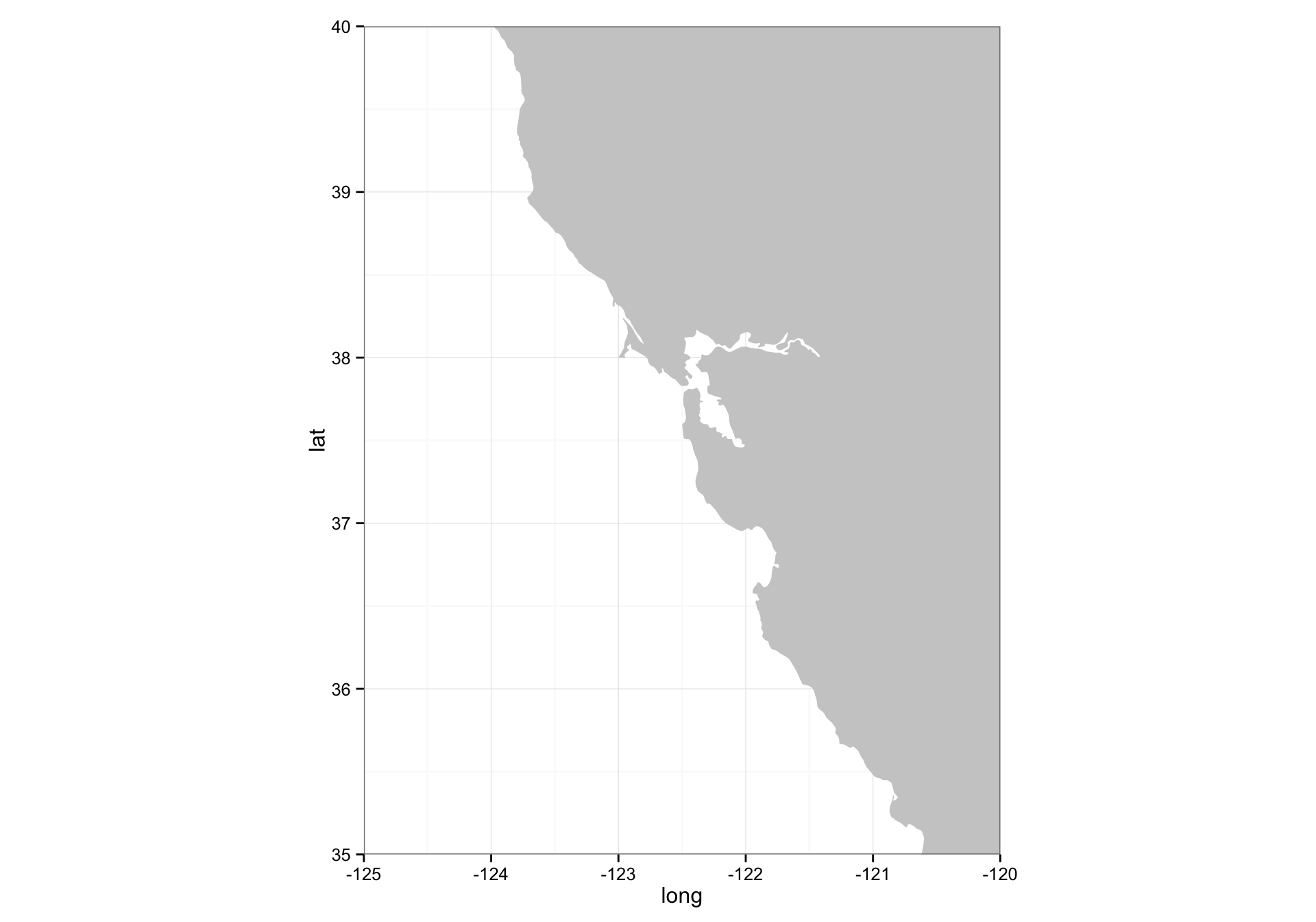
Let’s have a look at SF bay, first at a California scale:

w <- map_data("worldHires", ylim = c(35,40), xlim = c(-125,-120))
ggplot() + geom_polygon(data = w, aes(x=long, y = lat, group = group), fill = "grey80") + 
  coord_fixed(1.3, xlim = c(-125,-120), ylim = c(35,40)) + 
  theme_bw()

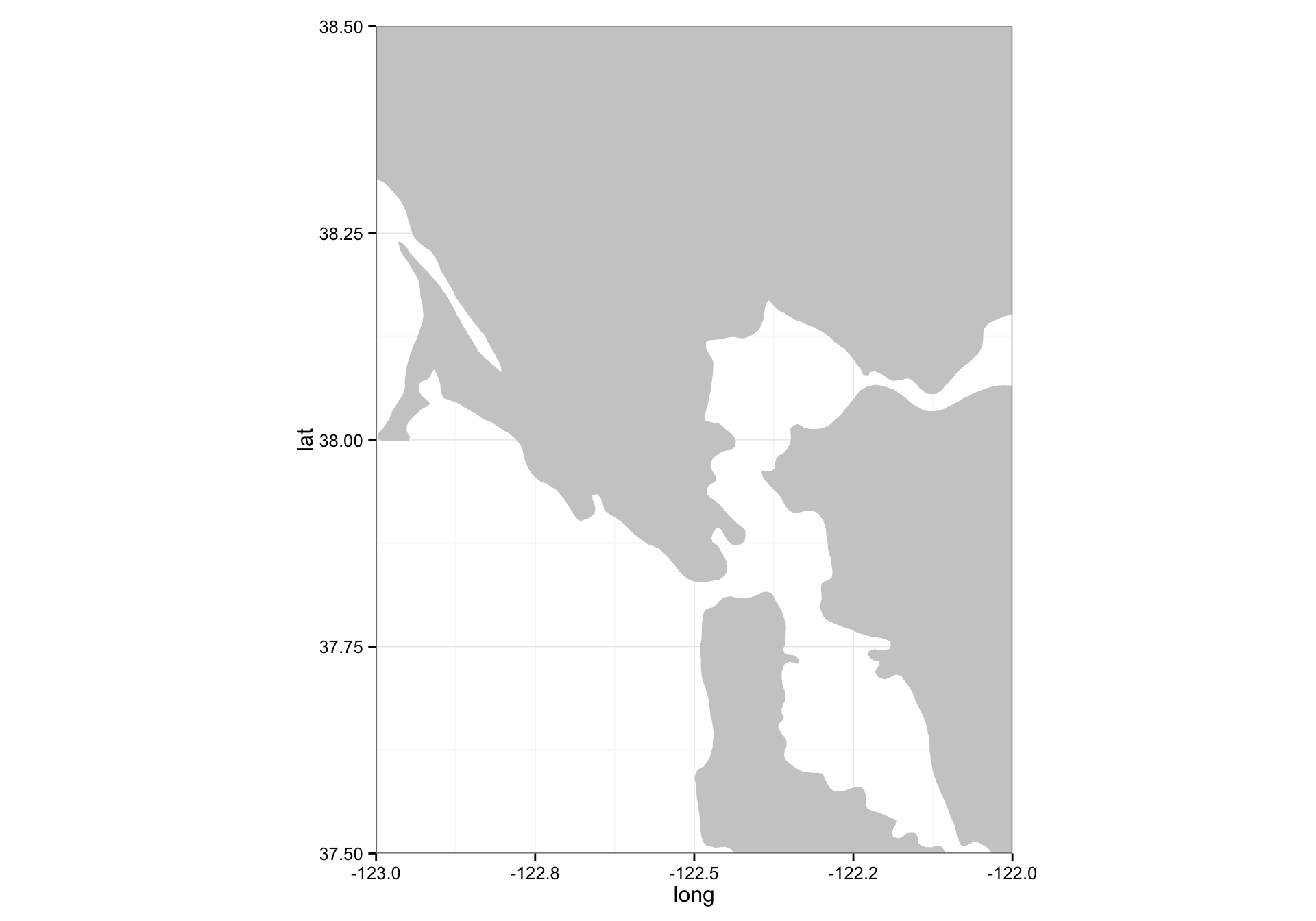
And then at a Bay scale:

ggplot() + geom_polygon(data = w, aes(x=long, y = lat, group = group), fill = "grey80") + 
  coord_fixed(1.3, xlim = c(-123,-122), ylim = c(37.5,38.5)) + 
  theme_bw()

And compare to GSHHS

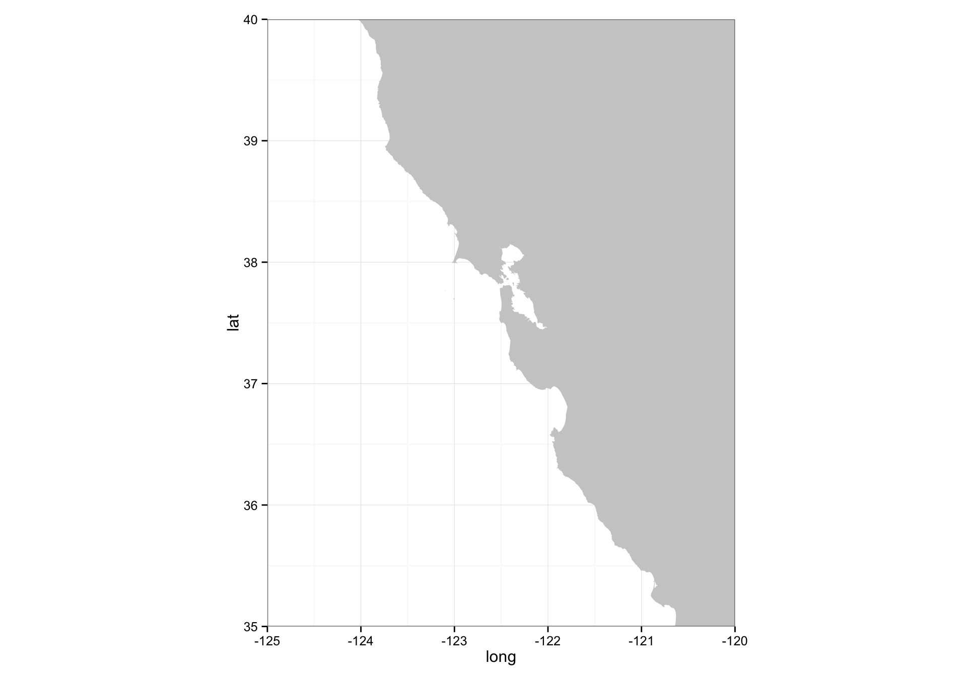
First at the California scale.

if (!rgeosStatus()) gpclibPermit()
gshhs.f.b <- "/Users/eriq/Maps/gshhg-bin-2.3.3/gshhs_f.b"
sf1 <- getRgshhsMap(gshhs.f.b, xlim = c(-125, -120), ylim = c(35, 40)) %>%
  fortify()

## Data are polygon data
## Data are polygon data
## Rgshhs: clipping 1 of 20 polygons ...

ggplot() + geom_polygon(data = sf1, aes(x=long, y = lat, group = group), fill = "grey80") + 
  coord_fixed(1.3, xlim = c(-125,-120), ylim = c(35,40)) + 
  theme_bw()

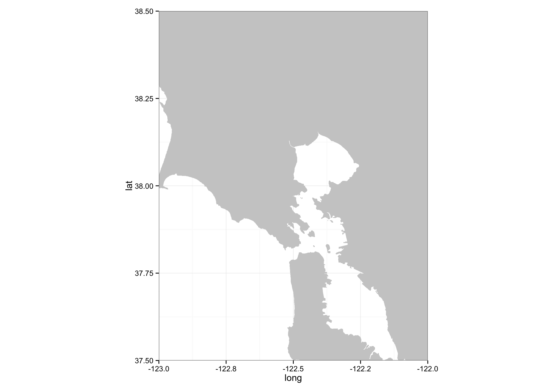
Then at the Bay scale:

ggplot() + geom_polygon(data = sf1, aes(x=long, y = lat, group = group), fill = "grey80") + 
  coord_fixed(1.3, xlim = c(-123,-122), ylim = c(37.5,38.5)) + 
  theme_bw()

OK. So the GSHHS at full resolution is clearly higher quality.

Another important thing to note

What is even more intriguing about this is that it appears that ``ggplot2's get_map function is not very good at grabbing just the part of the worldHires map that is requested. When you ask for the SF bay region it returns pretty much all of the USA, perhaps because that is all one polygon. On the other hand, when using getRgshhsMap it it appears that the function grabs just the area of interest and then appropriately closes the polygons. As a consequence, the GSHHS maps seems to plot a little faster using ggplot than the mapdata` map, and it takes up much less space in memory:

format(object.size(sf1), units = "Mb")

## [1] "0.3 Mb"

format(object.size(w), units = "Mb")

## [1] "2.5 Mb"

Let us add some rivers

I am curious to know at what scale the rivers are mapped to.

wdb_rivers_f.b <- "/Users/eriq/Maps/gshhg-bin-2.3.3/wdb_rivers_f.b"
rivers <- getRgshhsMap(wdb_rivers_f.b, xlim = c(-125, -120), ylim = c(35, 40)) 

## Data are line data
## Data are line data

oops! that is going to be harder to deal with…